Next: Gauge Symmetry in Quantum Up: Electrons in an Electromagnetic Previous: Review of the Classical Contents
We will quantize the Hamiltonian
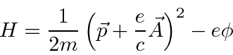
in the usual way, by replacing the momentum by the momentum operator, for the case of a constant magnetic field.
Note that the momentum operator will now include momentum in the field, not just the particle's momentum.
As this Hamiltonian is written,
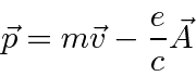
![]() is the variable conjugate to
is the variable conjugate to
![]() and is related to the velocity by
and is related to the velocity by
The
computation
yields

 compared to hydrogen binding energy),
and the second can be neglected.
The second term may be important in very high magnetic fields like those produced near
neutron stars or if distance scales are larger than in atoms like in a plasma (see example below).
compared to hydrogen binding energy),
and the second can be neglected.
The second term may be important in very high magnetic fields like those produced near
neutron stars or if distance scales are larger than in atoms like in a plasma (see example below).
So, for atoms, the dominant additional term is the one we anticipated classically
in section 18.4,
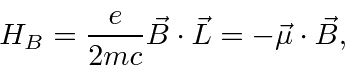
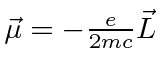 .
This is, effectively, the magnetic moment
due to the electron's orbital angular momentum.
In atoms, this term gives rise to the Zeeman effect: otherwise degenerate atomic states
split in energy when a magnetic field is applied.
Note that the electron spin which is not included here also contributes to the splitting and will
be studied later.
.
This is, effectively, the magnetic moment
due to the electron's orbital angular momentum.
In atoms, this term gives rise to the Zeeman effect: otherwise degenerate atomic states
split in energy when a magnetic field is applied.
Note that the electron spin which is not included here also contributes to the splitting and will
be studied later.
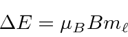
The Zeeman effect, neglecting electron spin, is particularly simple to calculate because the the hydrogen energy eigenstates are also eigenstates of the additional term in the Hamiltonian. Hence, the correction can be calculated exactly and easily.
* Example:
Splitting of orbital angular momentum states in a B field.*
The result is that the shifts in the eigen-energies are
The additional magnetic field terms are important in a plasma because the typical radii can be much bigger than in an atom. A plasma is composed of ions and electrons, together to make a (usually) electrically neutral mix. The charged particles are essentially free to move in the plasma. If we apply an external magnetic field, we have a quantum mechanics problem to solve. On earth, we use plasmas in magnetic fields for many things, including nuclear fusion reactors. Most regions of space contain plasmas and magnetic fields.
In the example below, we will solve the Quantum Mechanics problem two ways: one using our new Hamiltonian with B field terms, and the other writing the Hamiltonian in terms of A. The first one will exploit both rotational symmetry about the B field direction and translational symmetry along the B field direction. We will turn the radial equation into the equation we solved for Hydrogen. In the second solution, we will use translational symmetry along the B field direction as well as translational symmetry transverse to the B field. We will now turn the remaining 1D part of the Schrödinger equation into the 1D harmonic oscillator equation, showing that the two problems we have solved analytically are actually related to each other!
* Example:
A neutral plasma in a constant magnetic field.*
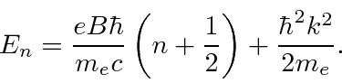
The result in either solution for the eigen-energies can be written as