The Classical Electromagnetic Field

For the study of the Maxwell field, it is most convenient to make a small modification to the system of units that are used. In Rationalized Heaviside-Lorentz Units the fields are all reduced by a factor of $\sqrt{4\pi}$ and the charges are increased by the same factor. With this change Maxwell's equations, as well as the Lagrangians we use, are simplified. It would have simplified many things if Maxwell had started off with this set of units.

As is well known from classical electricity and magnetism, the electric and magnetic field components are actually elements of a rank 2 Lorentz tensor.

$$\bgroup\color{black} F_{\mu\nu}=\pmatrix{ 0 & B_z & -B_y & -i... ...cr B_y & -B_x & 0 & -iE_z \cr iE_x & iE_y & iE_z & 0} \egroup$$

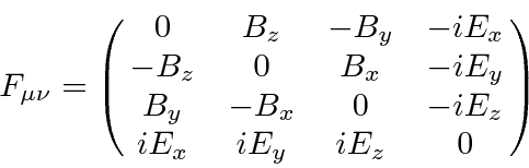
This field tensor can simply be written in terms of the vector potential, (which is a Lorentz vector).

$$\begin{eqnarray*} A_\mu&=&(\vec{A},i\phi) \\ F_{\mu\nu}&=&{\partial A_\nu\over\partial x_\mu}-{\partial A_\mu\over\partial x_\nu} \\ \end{eqnarray*}$$

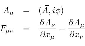
Note that $F_{\mu\nu}$ is automatically antisymmetric under the interchange of the indices.

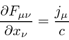
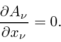
With the fields so derived from the vector potential, two of Maxwell's equations are automatically satisfied. The remaining two equations can be written as one 4-vector equation.

$$\bgroup\color{black} {\partial F_{\mu\nu}\over\partial x_\nu}={j_\mu\over c} \egroup$$

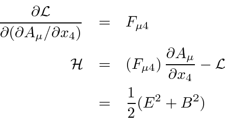
We now wish to pick a scalar Lagrangian. Since E&M is a well understood theory, the Lagrangian that is known to give the right equations is also known.

$$\bgroup\color{black} {\cal L}=-{1\over 4}F_{\mu\nu}F_{\mu\nu}+{1\over c}j_\mu A_\mu \egroup$$

Note that (apart from the speed of light not being set to 1) the Lagrangian does not contain needless constants in this set of units. The last term is a source term which provides the interaction between the EM field and charged particles. In working with this Lagrangian, we will treat each component of $A$ as an independent field. In this case, the Euler-Lagrange equation is Maxwell's equation as written above.

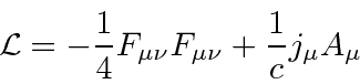
The free field Hamiltonian density can be computed according to the standard prescription yielding

$$\begin{eqnarray*} {\partial{\cal L}\over\partial(\partial A_\mu/\partial x_4)}&=... ... A_\mu\over\partial x_4}-{\cal L} \\ &=&{1\over 2}(E^2+B^2) \\ \end{eqnarray*}$$

if there are no source terms in the region.

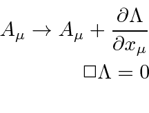
Gauge symmetry may be used to put a condition on the vector potential.

$$\bgroup\color{black} {\partial A_\nu\over\partial x_\nu}=0. \egroup$$

This is called the Lorentz condition. Even with this satisfied, there is still substantial gauge freedom possible. Gauge transformations can be made as shown below.

$$\begin{eqnarray*} A_\mu\rightarrow A_\mu+{\partial\Lambda\over\partial x_\mu} \\ \Box\Lambda=0 \\ \end{eqnarray*}$$