Next: The Potential Barrier Up: Piecewise Constant Potentials in Previous: The Potential Well with Contents
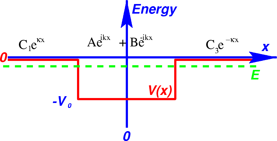
We will work with the same potential well as in the previous section but assume that
 ,
making this a bound state problem.
Note that this potential has a Parity symmetry.
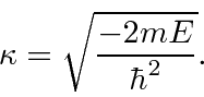
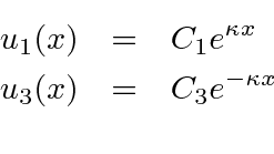
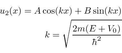
In the left and right regions the general solution is
,
making this a bound state problem.
Note that this potential has a Parity symmetry.
In the left and right regions the general solution is

 and
the
and
the
 since they diverge
and we could never normalize to one bound particle.
since they diverge
and we could never normalize to one bound particle.
The
calculation
shows that either
![]() or
or
![]() must be zero for a solution.
This means that the solutions separate into even parity and odd parity states.
We could have guessed this from the potential.
must be zero for a solution.
This means that the solutions separate into even parity and odd parity states.
We could have guessed this from the potential.
The even states have the (quantization) constraint on the energy that
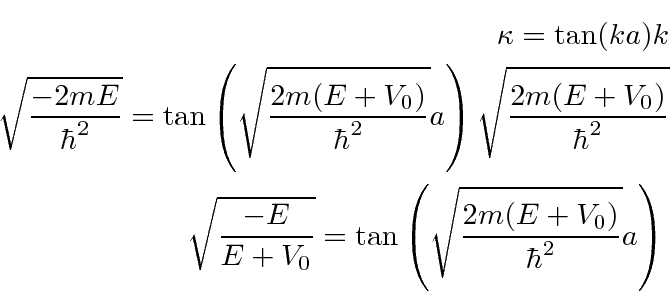
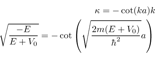
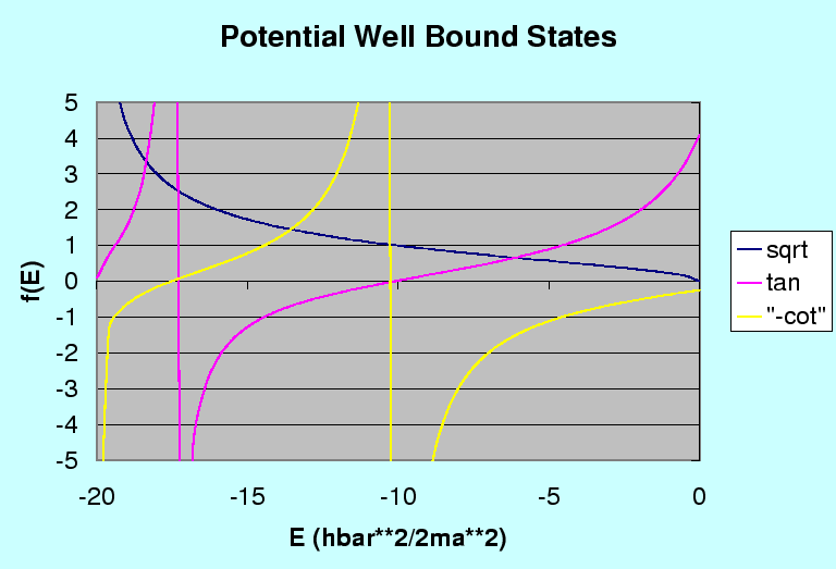
These are transcendental equations, so we will solve them graphically. The plot below compares the square root on the left hand side of the transcendental equations to the tangent on the right for the event states and to ``-cotangent'' on the right for odd states. Where the curves intersect (not including the asymptote), is an allowed energy. There is always one even solution for the 1D potential well. In the graph shown, there are 2 even and one odd solution. The wider and deeper the well, the more solutions.
Try this 1D Potential Applet. It allows you to vary the potential and see the eigenstates.