Next: Resonant Scattering Up: Quantum Physics 130 Previous: Black Body Radiation Spectrum Contents
The scattering process clearly requires terms in
 that annihilate one photon and create another.
The order does not matter.
The
that annihilate one photon and create another.
The order does not matter.
The
 is the square of the Fourier decomposition of the
radiation field so it contains terms like
is the square of the Fourier decomposition of the
radiation field so it contains terms like
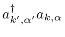 and
and
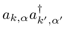 which are just what we want.
The
which are just what we want.
The
 term has both creation and annihilation operators in it but not
products of them.
It changes the number of photons by plus or minus one, not by zero as required for the scattering process.
Nevertheless this part of the interaction could contribute in second order perturbation theory,
by absorbing one photon in a transition from the initial atomic state to an intermediate state,
then emitting another photon and making a transition to the final atomic state.
While this is higher order in perturbation theory, it is the same order in the electromagnetic coupling constant
term has both creation and annihilation operators in it but not
products of them.
It changes the number of photons by plus or minus one, not by zero as required for the scattering process.
Nevertheless this part of the interaction could contribute in second order perturbation theory,
by absorbing one photon in a transition from the initial atomic state to an intermediate state,
then emitting another photon and making a transition to the final atomic state.
While this is higher order in perturbation theory, it is the same order in the electromagnetic coupling constant
![]() ,
which is what really counts when expanding in powers of
,
which is what really counts when expanding in powers of
![]() .
Therefore, we will need to consider the
.
Therefore, we will need to consider the
 term in first order and
the
term in first order and
the
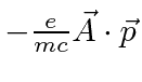 term in second order perturbation theory
to get an order
term in second order perturbation theory
to get an order
![]() calculation of the matrix element.
calculation of the matrix element.
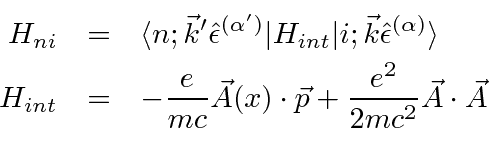
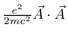
Start with the first order perturbation theory term.
All the terms in the sum that do not annihilate the initial state photon and create the final state photon give zero.
We will assume that the wavelength of the photon's is long compared to the size of the atom so that
![]() .
.
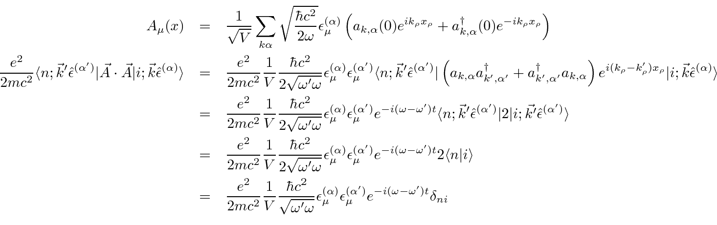
This is the matrix element
 .
The amplitude to be in the final state
.
The amplitude to be in the final state
 is given by first order
time dependent perturbation theory.
is given by first order
time dependent perturbation theory.
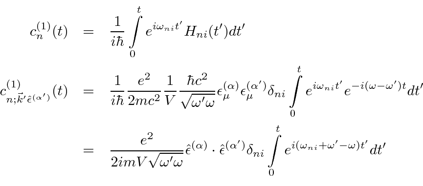
 .
We will carry along the integral for now, since we are not yet ready to square it.
.
We will carry along the integral for now, since we are not yet ready to square it.
Now we very carefully put the interaction term
into the formula for second order time dependent perturbation theory, again using
![]() .
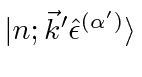
Our notation is that the
intermediate state of atom and field is called
.
Our notation is that the
intermediate state of atom and field is called
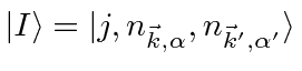 where
where
![]() represents the state of the atom and we may have zero or two photons, as indicated in the diagram.
represents the state of the atom and we may have zero or two photons, as indicated in the diagram.
The space-time diagram below shows the three terms in
 Time is assumed to run upward in the diagrams.
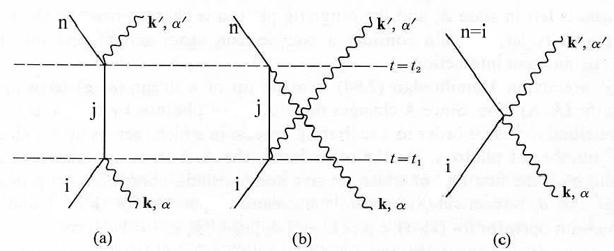
Looking again at the formula for the second order scattering amplitude,
note that we integrate over the times
![]() and
and
![]() and that
and that
 .
For diagram (a), the annihilation operator
.
For diagram (a), the annihilation operator
 is active at time
![]() and the creation operator is active at time
and the creation operator is active at time
![]() .
For diagram (b) its just the opposite.
The second order formula above contains four terms as written.
The
.
For diagram (b) its just the opposite.
The second order formula above contains four terms as written.
The
![]() and
and
![]() terms are the ones described by the diagram.
The
terms are the ones described by the diagram.
The
![]() and
and
![]() terms will clearly give zero.
Note that we are just picking the terms that will survive the calculation,
not changing any formulas.
terms will clearly give zero.
Note that we are just picking the terms that will survive the calculation,
not changing any formulas.
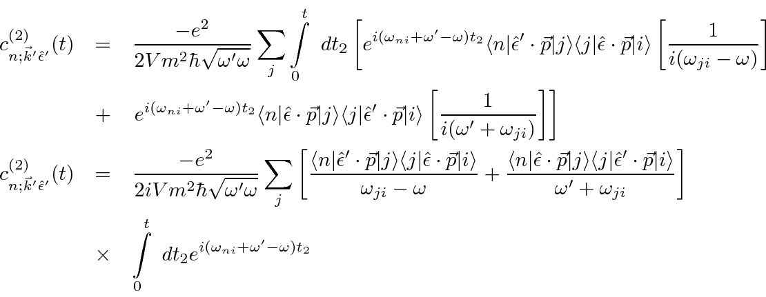
Now, reduce to the two nonzero terms.
The operators just give a factor of
![]() and make the photon states work out.
If
and make the photon states work out.
If
![]() is the intermediate atomic state, the second order term reduces to.
is the intermediate atomic state, the second order term reduces to.
![\begin{eqnarray*}
c_{n;\vec{k}'\hat{\epsilon}^{(\alpha')}}^{(2)}(t)
&=&{-e^2\ove...
...mega_{ji})t_2}-1\over i(\omega'+\omega_{ji})}\right]
\right] \\
\end{eqnarray*}](img4051.png)
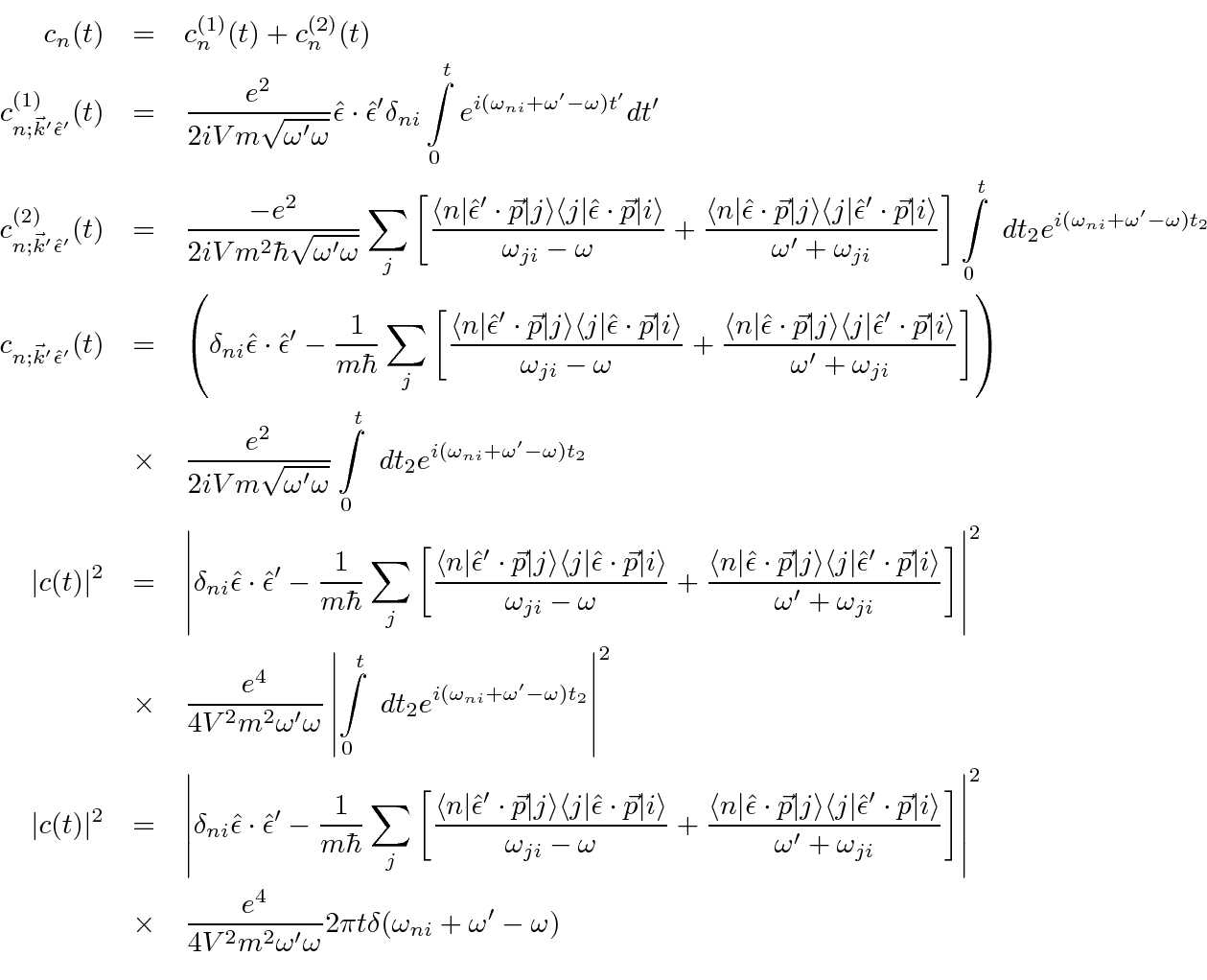
We have calculated all the amplitudes. The first order and second order amplitudes should be combined, then squared.
![\begin{eqnarray*}
\Gamma
&=& \int{Vd^3k'\over (2\pi)^3} \left\vert
\delta_{ni} \...
...t i\rangle
\over \omega'+\omega_{ji}}
\right] \right\vert^2 \\
\end{eqnarray*}](img4055.png)
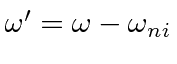 ,
but we have left
,
but we have left
The final step to a differential cross section is to divide the transition rate by the
incident flux of particles.
This is a surprisingly easy step because we are using plane waves of photons.
The initial state is one particle in the volume ![]() moving with a velocity of
moving with a velocity of ![]() ,
so the flux is simply
,
so the flux is simply
![]() .
.
![\begin{displaymath}\bgroup\color{black} {d\sigma\over d\Omega}
= {e^4\omega'\ove...
...angle
\over \omega'+\omega_{ji}}
\right] \right\vert^2 \egroup\end{displaymath}](img4060.png)
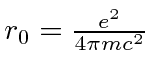 in our units.
We will factor the square of this out but leave the answer in terms of fundamental constants.
in our units.
We will factor the square of this out but leave the answer in terms of fundamental constants.
![\begin{displaymath}\bgroup\color{black} {d\sigma\over d\Omega}
= \left({e^2\over...
...angle
\over \omega_{ji}+\omega'}
\right] \right\vert^2 \egroup\end{displaymath}](img464.png)
 .)
Note that, for the very short time that the system is in an intermediate state,
energy conservation is not strictly enforced.
The energy denominators in the formula suppress larger energy non-conservation.
The formula can be applied to several physical situations as discussed below.
.)
Note that, for the very short time that the system is in an intermediate state,
energy conservation is not strictly enforced.
The energy denominators in the formula suppress larger energy non-conservation.
The formula can be applied to several physical situations as discussed below.
Also note that the formula yields an infinite result if
 .
This is not a physical result.
In fact the cross section will be large but not infinite when energy is conserved in the intermediate state.
This condition is often refereed to as ``the intermediate state being on the mass shell'' because
of the relation between energy and mass in four dimensions.
.
This is not a physical result.
In fact the cross section will be large but not infinite when energy is conserved in the intermediate state.
This condition is often refereed to as ``the intermediate state being on the mass shell'' because
of the relation between energy and mass in four dimensions.