Next: The Dirac Equation Up: Course Summary Previous: Electron Self Energy Contents
![\begin{displaymath}\bgroup\color{black} H={1\over 2m}\left(\vec{\sigma}\cdot[\ve...
...{e\over c}\vec{A}(\vec{r},t)]\right)^2-e\phi(\vec{r},t) \egroup\end{displaymath}](img482.png)
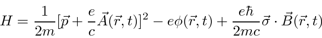
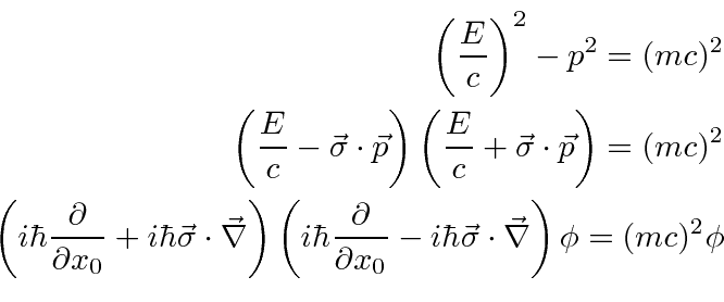
We can extend this concept to use the relativistic energy equation.
The idea is to replace
![]() with
with
 in the relativistic energy equation.
 and
and
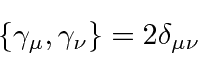
 and ordering it as a matrix equation, we get an equation that can be written as a dot product between 4-vectors.
![\begin{eqnarray*}
\pmatrix{-i\hbar{\partial\over\partial x_0} & -i\hbar\vec{\sig...
...]
=\hbar\left[\gamma_\mu{\partial\over\partial x_\mu}\right] \\
\end{eqnarray*}](img489.png)
 |
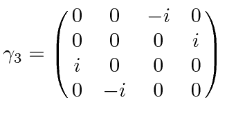 |
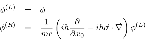
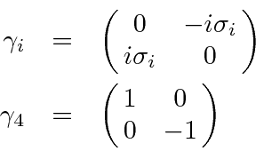
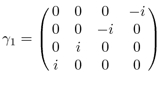
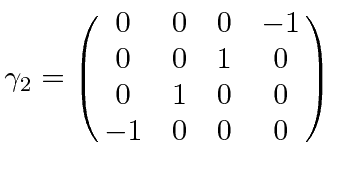
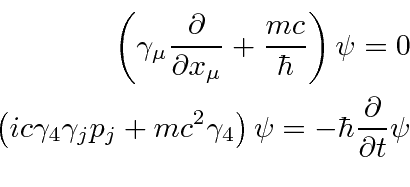
Defining
 ,
,
 .
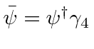
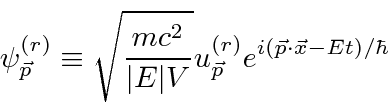
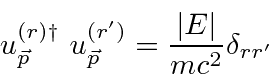
This indicates that the normalization of the state includes all four components of the Dirac spinors.
.
This indicates that the normalization of the state includes all four components of the Dirac spinors.
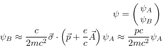
For non-relativistic electrons, the first two components of the Dirac spinor are large while the last two are small.
For a free particle, each component of the Dirac spinor satisfies the Klein-Gordon equation.
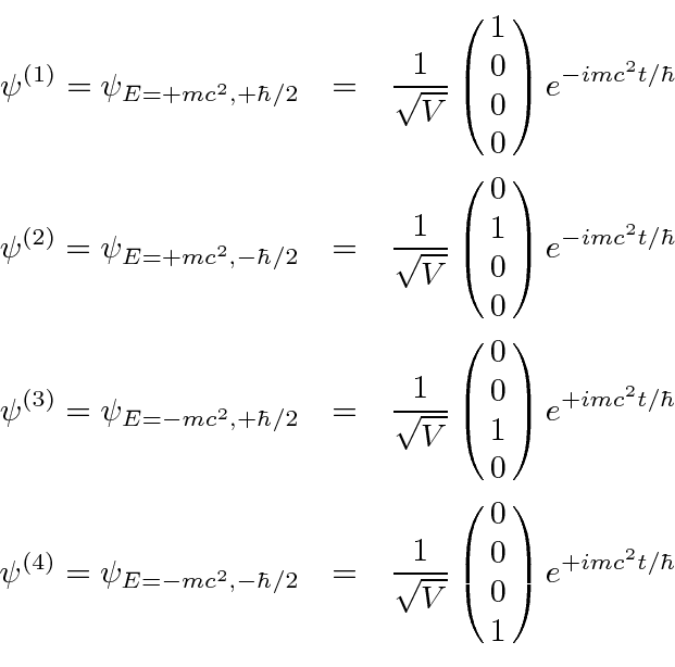
The four normalized solutions for a Dirac particle at rest are.
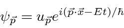
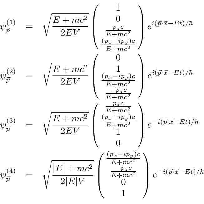
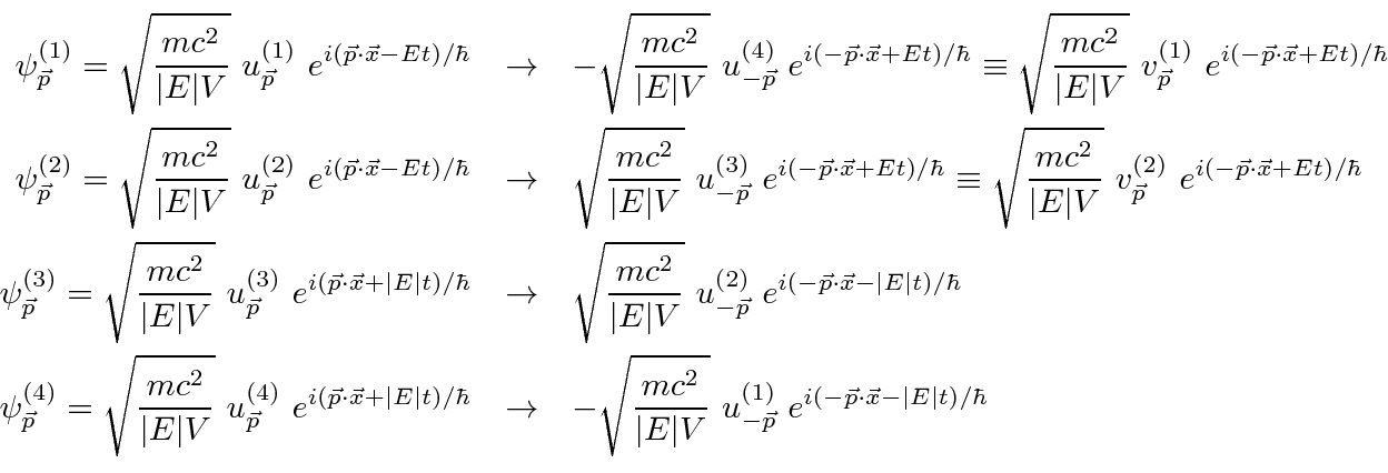
The next step is to find the solutions with definite momentum.
The four plane wave solutions to the Dirac equation are
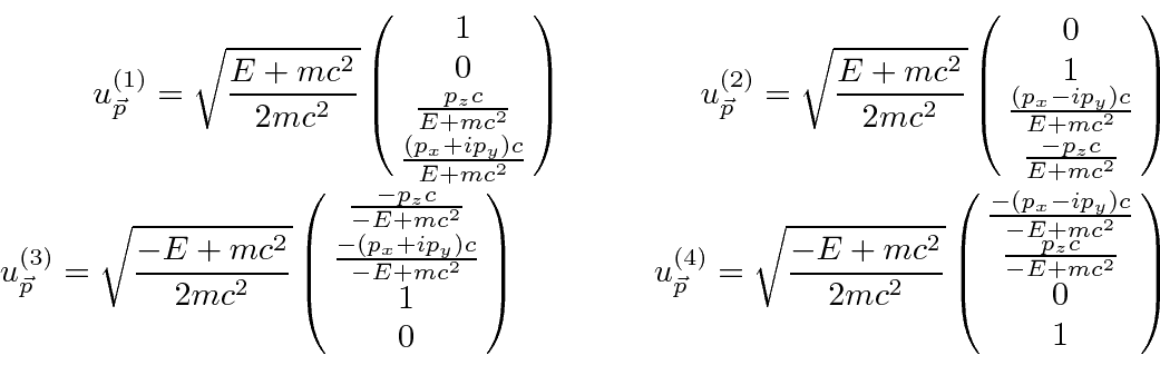
The solutions are not in general eigenstates of any component of spin but are eigenstates of helicity, the component of spin along the direction of the momentum.
Note that with
![]() negative, the exponential
negative, the exponential
![]() has the phase velocity,
the group velocity and the probability flux all in the opposite direction of the momentum as we have defined it.
This clearly doesn't make sense.
Solutions 3 and 4 need to be understood in a way for which the non-relativistic operators have not prepared us.
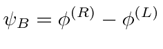
Let us simply relabel solutions 3 and 4 such that
has the phase velocity,
the group velocity and the probability flux all in the opposite direction of the momentum as we have defined it.
This clearly doesn't make sense.
Solutions 3 and 4 need to be understood in a way for which the non-relativistic operators have not prepared us.
Let us simply relabel solutions 3 and 4 such that
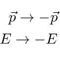
If we change the charge on the electron from
![]() to
to
![]() and change the sign of the exponent, the Dirac equation
remains the invariant.
Thus, we can turn the negative exponent solution (going backward in time) into the conventional positive exponent
solution if we change the charge to
and change the sign of the exponent, the Dirac equation
remains the invariant.
Thus, we can turn the negative exponent solution (going backward in time) into the conventional positive exponent
solution if we change the charge to
![]() .
We can interpret solutions 3 and 4 as positrons.
We will make this switch more carefully when we study the charge conjugation operator.
.
We can interpret solutions 3 and 4 as positrons.
We will make this switch more carefully when we study the charge conjugation operator.
The Dirac equation should be invariant under Lorentz boosts and under rotations,
both of which are just changes in the definition of an inertial coordinate system.
Under Lorentz boosts,
 transforms like a 4-vector but the
![]() matrices are constant.
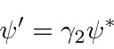
The Dirac equation is shown to be invariant under boosts along the
matrices are constant.
The Dirac equation is shown to be invariant under boosts along the
![]() direction
if we transform the Dirac spinor according to
direction
if we transform the Dirac spinor according to

 .
.
The
Dirac equation is invariant under rotations about the
![]() axis
if we transform the Dirac spinor according to
axis
if we transform the Dirac spinor according to
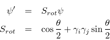
 is a cyclic permutation.
Another symmetry related to the choice of coordinate system is parity.
Under a parity inversion operation the Dirac equation remains invariant if
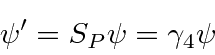
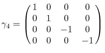 ,
the third and fourth components of the spinor change sign while the first two don't.
Since we could have chosen
,
the third and fourth components of the spinor change sign while the first two don't.
Since we could have chosen
 , all we know is that
components 3 and 4 have the opposite parity of components 1 and 2.
, all we know is that
components 3 and 4 have the opposite parity of components 1 and 2.
From 4 by 4 matrices, we may derive 16 independent components of covariant objects.
We define the product of all gamma matrices.
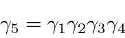
 .
.
The simplest set of covariants we can make from Dirac spinors and
![]() matrices are tabulated below.
matrices are tabulated below.
| Classification | Covariant Form | no. of Components |
| Scalar |
 |
1 |
| Pseudoscalar |
 |
1 |
| Vector |
 |
4 |
| Axial Vector |
 |
4 |
| Rank 2 antisymmetric tensor |
 |
6 |
| Total | 16 |
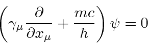
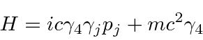
For many purposes, it is useful to write the Dirac equation in the traditional form
 .
To do this, we must separate the space and time derivatives, making the equation less covariant looking.
.
To do this, we must separate the space and time derivatives, making the equation less covariant looking.
Its easy to see the
![]() commutes with the Hamiltonian for a free particle so that momentum will be conserved.
The components of orbital angular momentum do not commute with
commutes with the Hamiltonian for a free particle so that momentum will be conserved.
The components of orbital angular momentum do not commute with
![]() .
.
![\begin{displaymath}\bgroup\color{black} [H,L_z]=ic\gamma_4[\gamma_jp_j,xp_y-yp_x]=\hbar c\gamma_4(\gamma_1p_y-\gamma_2 p_x) \egroup\end{displaymath}](img539.png)
![\begin{displaymath}\bgroup\color{black} {[H,S_z]}=\hbar c\gamma_4[\gamma_2p_x-\gamma_1p_y] \egroup\end{displaymath}](img540.png)
![\begin{eqnarray*}[H,J_z]=[H,L_z]+[H,S_z]=\hbar c\gamma_4(\gamma_1p_y-\gamma_2 p_x)+\hbar c\gamma_4[\gamma_2p_x-\gamma_1p_y]=0 \\
\end{eqnarray*}](img541.png)
We can also see that the helicity, or spin along the direction of motion does commute.
![\begin{displaymath}\bgroup\color{black} [H,\vec{S}\cdot\vec{p}]=[H,\vec{S}]\cdot\vec{p}=0 \egroup\end{displaymath}](img542.png)
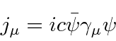
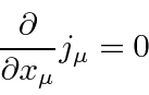
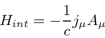
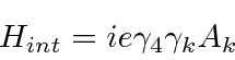
For any calculation, we need to know the interaction term with the Electromagnetic field.
Based on the interaction of field with a current
The Dirac equation has some unexpected phenomena which we can derive.
Velocity eigenvalues for electrons are always
![]() along any direction.
Thus the only values of velocity that we could measure are
along any direction.
Thus the only values of velocity that we could measure are
![]() .
.
Localized states, expanded in plane waves, contain all four components of the plane wave solutions. Mixing components 1 and 2 with components 3 and 4 gives rise to Zitterbewegung, the very rapid oscillation of an electrons velocity and position.
![\begin{eqnarray*}
\langle v_k\rangle&=&\sum\limits_{\vec{p}}\sum\limits_{r=1}^4\...
...mma_k u^{(r')}_{\vec{p}} e^{2i\vert E\vert t/\hbar}\right] \\
\end{eqnarray*}](img546.png)
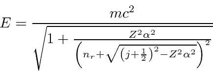
It is possible to solve the Dirac equation exactly for Hydrogen in a way very similar to the non-relativistic solution.
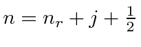
One difference is that it is clear from the beginning that the total angular momentum is a constant of the motion and
is used as a basic quantum number.
There is another conserved quantum number related to the component of spin along the direction of
![]() .
With these quantum numbers, the radial equation can be solved in a similar way as for the non-relativistic case
yielding the energy relation.
.
With these quantum numbers, the radial equation can be solved in a similar way as for the non-relativistic case
yielding the energy relation.
 .
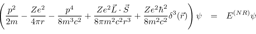
This result gives the same answer as our non-relativistic calculation to order
.
This result gives the same answer as our non-relativistic calculation to order
A calculation of Thomson scattering shows that even simple low energy photon scattering relies on the ``negative energy'' or positron states to get a non-zero answer. If the calculation is done with the two diagrams in which a photon is absorbed then emitted by an electron (and vice-versa) the result is zero at low energy because the interaction Hamiltonian connects the first and second plane wave states with the third and fourth at zero momentum. This is in contradiction to the classical and non-relativistic calculations as well as measurement. There are additional diagrams if we consider the possibility that the photon can create and electron positron pair which annihilates with the initial electron emitting a photon (or with the initial and final photons swapped). These two terms give the right answer. The calculation of Thomson scattering makes it clear that we cannot ignore the new ``negative energy'' or positron states.
The Dirac equation is invariant under charge conjugation, defined as changing electron states into the opposite charged
positron states with the same momentum and spin (and changing the sign of external fields).
To do this the Dirac spinor is transformed according to.
 and
and
 that are charge conjugates of
 and
and
 .
.
Jim Branson 2013-04-22