Next: Explicit 2p to 1s Up: Radiation in Atoms Previous: Total Decay Rate Using Contents
 term to allow us to compute matrix elements more easily.
Since
term to allow us to compute matrix elements more easily.
Since
 and the matrix element is squared,
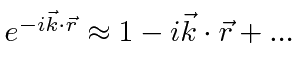
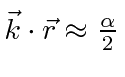
our expansion will be in powers of
and the matrix element is squared,
our expansion will be in powers of
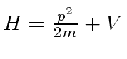
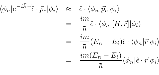
In this Electric Dipole approximation, we can make general progress on computation of the matrix element.
If the Hamiltonian is of the form
 and
and
![\bgroup\color{black}$[V,\vec{r}]=0$\egroup](img3585.png) , then
, then
![\begin{displaymath}\bgroup\color{black} [H,\vec{r}]={\hbar\over i}{p\over m} \egroup\end{displaymath}](img3586.png)
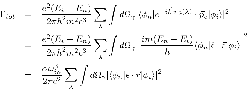
![\bgroup\color{black}$\vec{p}={im\over\hbar}[H,\vec{r}]$\egroup](img3587.png) in terms of the commutator.
in terms of the commutator.
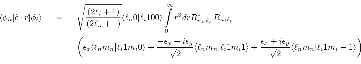
We can proceed further, with the angular part of the (matrix element) integral.
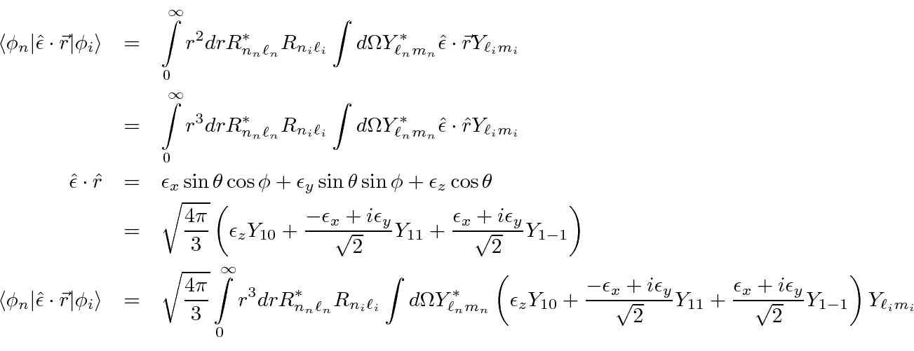
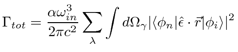
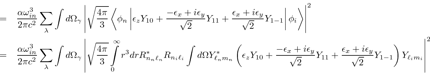
At this point, lets bring all the terms in the formula back together so we know what we are doing.
 |
 for the sake of modularity of the calculation.
The integral with three spherical harmonics in each term looks a bit difficult, but,
we can use a Clebsch-Gordan series like the one in addition of angular momentumto help us solve the problem.
We will write the product of two spherical harmonics in terms of a sum of spherical harmonics.
Its very similar to adding the angular momentum from the two
![]() s.
Its the same series as we had for addition of angular momentum (up to a constant).
(Note that things will be very simple if either the initial or the final state have
s.
Its the same series as we had for addition of angular momentum (up to a constant).
(Note that things will be very simple if either the initial or the final state have
![]() ,
a case we will work out below for transitions to s states.)
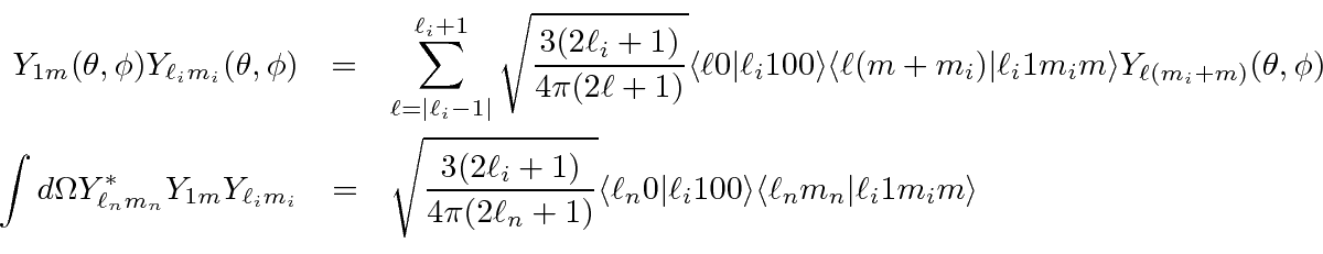
The general formula for rewriting the product of two spherical harmonics (which are functions of the same coordinates) is
,
a case we will work out below for transitions to s states.)
The general formula for rewriting the product of two spherical harmonics (which are functions of the same coordinates) is

 can be thought of as a normalization constant in
an otherwise normal Clebsch-Gordan series.
(Note that the normal addition of the orbital angular momenta of two particles would have product states
of two spherical harmonics in different coordinates, the coordinates of particle one and of particle two.)
(The derivation of the above equation involves a somewhat detailed study of the properties of rotation matrices
and would take us pretty far off the current track (See Merzbacher page 396).)
can be thought of as a normalization constant in
an otherwise normal Clebsch-Gordan series.
(Note that the normal addition of the orbital angular momenta of two particles would have product states
of two spherical harmonics in different coordinates, the coordinates of particle one and of particle two.)
(The derivation of the above equation involves a somewhat detailed study of the properties of rotation matrices
and would take us pretty far off the current track (See Merzbacher page 396).)
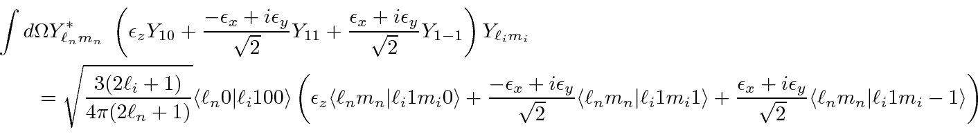
First add the angular momentum from the initial state
 and the photon
 using the Clebsch-Gordan series,
with the usual notation for the Clebsch-Gordan coefficients
using the Clebsch-Gordan series,
with the usual notation for the Clebsch-Gordan coefficients
 .
.
I remind you that the Clebsch-Gordan coefficients in these equations are just numbers which are less than one. They can often be shown to be zero if the angular momentum doesn't add up. The equation we derive can be used to give us a great deal of information.
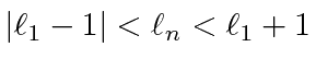 so the change in in
 .
For other values, all the Clebsch-Gordan coefficients above will be zero.
.
For other values, all the Clebsch-Gordan coefficients above will be zero.
We also know that the
 are odd under parity so the other two spherical harmonics must have opposite parity to
each other implying that
are odd under parity so the other two spherical harmonics must have opposite parity to
each other implying that
 , therefore
We also know from the addition of angular momentum that the z components just add like integers, so the three
Clebsch-Gordan coefficients allow
We can also easily note that we have no operators which can change the spin here.
So certainly
The above selection rules apply only for the Electric Dipole (E1) approximation.
Higher order terms in the expansion, like the Electric Quadrupole (E2) or the Magnetic Dipole (M1),
allow other decays but the rates are down by a factor of
![]() or more.
There is one absolute selection rule coming from angular momentum conservation, since the photon is spin 1.
No
or more.
There is one absolute selection rule coming from angular momentum conservation, since the photon is spin 1.
No  to transitions in any order of approximation.
As a summary of our calculations in the Electric Dipole approximation, lets write out the decay rate formula.
Jim Branson 2013-04-22