Next: Examples Up: Time Dependent Perturbation Theory Previous: General Time Dependent Perturbations Contents

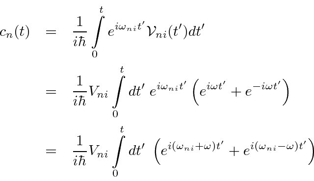
Putting this perturbation into the expression for
 , we get
For
![]() , the time integral of the exponential gives (some kind of)
delta function of energy conservation.
We will expend some effort to determine exactly what delta function it is.
, the time integral of the exponential gives (some kind of)
delta function of energy conservation.
We will expend some effort to determine exactly what delta function it is.
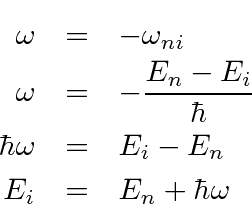
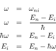
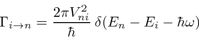
Lets take the case of radiation of an energy quantum
![]() .
If the initial and final states have energies such that this transition goes,
the absorption term is completely negligible.
(We can just use one of the exponentials at a time to make our formulas simpler.)
.
If the initial and final states have energies such that this transition goes,
the absorption term is completely negligible.
(We can just use one of the exponentials at a time to make our formulas simpler.)
The amplitude to be in state
![]() as a function of time is
as a function of time is
![\begin{eqnarray*}
c_n(t)
&=&{1\over i\hbar}V_{ni}\int\limits_0^tdt'\;e^{i(\omeg...
...ega_{ni}+\omega) t/2\right)\over (\omega_{ni}+\omega)^2}\right]
\end{eqnarray*}](img3529.png)
 which can be a VERY short time),
the term in square brackets looks like some kind of delta function.
which can be a VERY short time),
the term in square brackets looks like some kind of delta function.
We will
show
that the quantity in square brackets in the last equation is
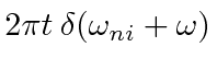 .
The probability to be in state
.
The probability to be in state
![]() then is
then is

Since the probability to be in the final state increases linearly with time, it is reasonable to describe this in terms of a transition rate. The transition rate is then given by
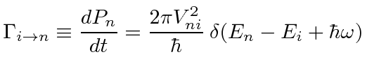 |
It does not make a lot of sense to use this equation with a delta function to calculate the transition rate from a discrete state to a discrete state. If we tune the frequency just right we get infinity otherwise we get zero. This formula is what we need if either the initial or final state is a continuum state. If there is a free particle in the initial state or the final state, we have a continuum state. So, the absorption or emission of a particle, satisfies this condition.
The above results are very close to a transition rate formula known as Fermi's Golden Rule.
Imagine that instead of one final state
![]() there are a continuum of final states.
The total rate to that continuum would be obtained by integrating over final state energy,
an integral done simply with the delta function.
We then have
there are a continuum of final states.
The total rate to that continuum would be obtained by integrating over final state energy,
an integral done simply with the delta function.
We then have
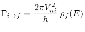 |
 is the density of final states.
When particles (like photons or electrons) are emitted, the final state will
be a continuum due to the continuum of states available to a free particle.
We will need to carefully compute the density of those states, often known as phase space.
is the density of final states.
When particles (like photons or electrons) are emitted, the final state will
be a continuum due to the continuum of states available to a free particle.
We will need to carefully compute the density of those states, often known as phase space.