Next: Derivation of 1st Order Up: Derivations and Computations Previous: Derivations and Computations Contents
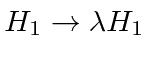
To keep track of powers of the perturbation in this derivation we will make the substitution
 where
where
![]() is assumed to be a small parameter in which we are making the series expansion of our
energy eigenvalues and eigenstates.
It is there to do the book-keeping correctly and can go away at the end of the derivations.
is assumed to be a small parameter in which we are making the series expansion of our
energy eigenvalues and eigenstates.
It is there to do the book-keeping correctly and can go away at the end of the derivations.
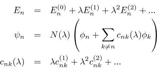
To solve the problem using a perturbation series,
we will expand both our energy eigenvalues and eigenstates in powers of
![]() .
.
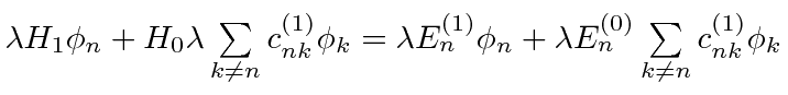
The full Schrödinger equation is
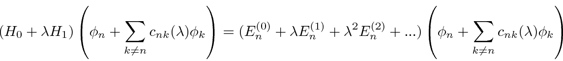
 has been factored out on both sides.
For this equation to hold as we vary
has been factored out on both sides.
For this equation to hold as we vary
|
|
 |
|
|
 |
|
|
 |
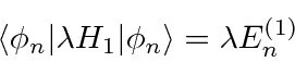
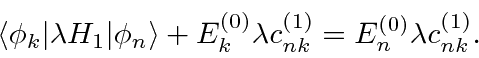
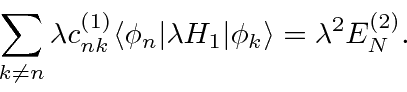
The first order equation dotted into
![]() yields
yields
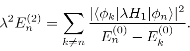
The second order equation projected on
![]() yields
yields
 , we have
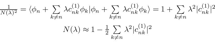
The normalization factor
played no role in the solutions to the Schrödinger
equation since that equation is independent of normalization.
We do need to go back and check whether the first order
corrected wavefunction needs normalization.
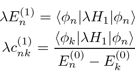
These results are rewritten with all the
![]() removed in section 22.1.
removed in section 22.1.