Next: The Same Problem with Up: Eigenfunctions, Eigenvalues and Vector Previous: Eigenfunctions and Vector Space Contents
As a simple example, we will solve the 1D Particle in a Box problem.
That is a particle confined to a region
 .
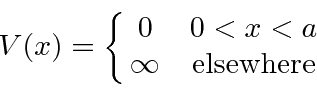
We can do this with the (unphysical) potential which is zero with in those limits and
.
We can do this with the (unphysical) potential which is zero with in those limits and
 outside the limits.
Because of the infinite potential, this problem has very
unusual boundary conditions.
(Normally we will require continuity of the wave function and its first derivative.)
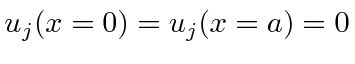
The wave function must be zero at
![]() and
and
![]() since it must be continuous and it
is zero in the region of infinite potential.
The first derivative does not need to be continuous at the boundary (unlike other problems),
because of the infinite discontinuity in the potential.
since it must be continuous and it
is zero in the region of infinite potential.
The first derivative does not need to be continuous at the boundary (unlike other problems),
because of the infinite discontinuity in the potential.
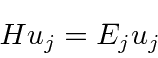
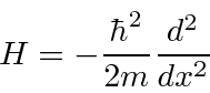
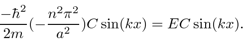
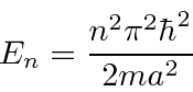
The time independent Schrödinger equation
(also called the energy eigenvalue equation) is

The solution inside the box could be written as
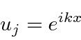
 .
.
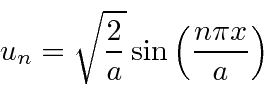
We can do this easily by choosing
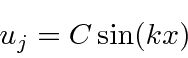
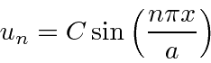
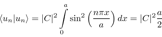
We have solutions to the Schrödinger equation that satisfy the boundary conditions.
Now we need to set the constant
![]() to normalize them to 1.
to normalize them to 1.
The first four eigenfunctions are graphed below. The ground state has the least curvature and the fewest zeros of the wavefunction.
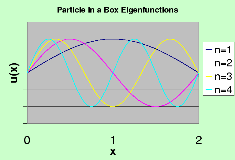
Note that these states would have a definite parity if
![]() were at the center of the box.
were at the center of the box.
The expansion of an arbitrary wave function in these eigenfunctions is essentially our original Fourier Series. This is a good example of the energy eigenfunctions being orthogonal and covering the space.