Next: The Lamb Shift Up: Quantum Physics 130 Previous: Raman Effect Contents
 .
Experiments have probed the electron's charge distribution and found that it is consistent with a point
charge down to distances much smaller than the classical radius.
Beyond classical calculations, the
self energy of the electron calculated in the quantum theory of Dirac is still infinite
but the divergences are less severe.
.
Experiments have probed the electron's charge distribution and found that it is consistent with a point
charge down to distances much smaller than the classical radius.
Beyond classical calculations, the
self energy of the electron calculated in the quantum theory of Dirac is still infinite
but the divergences are less severe.
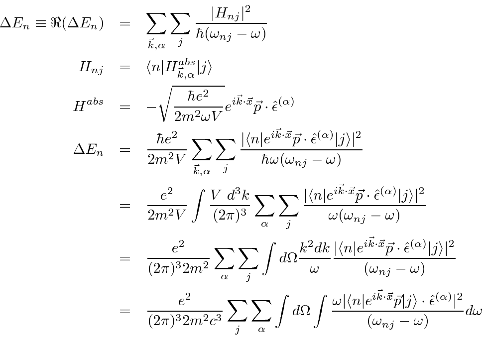
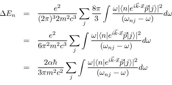
At this point we must take the unpleasant position that this (constant) infinite energy should just be subtracted when we consider the overall zero of energy (as we did for the field energy in the vacuum). Electrons exist and don't carry infinite amount of energy baggage so we just subtract off the infinite constant. Nevertheless, we will find that the electron's self energy may change when it is a bound state and that we should account for this change in our energy level calculations. This calculation will also give us the opportunity to understand resonant behavior in scattering.
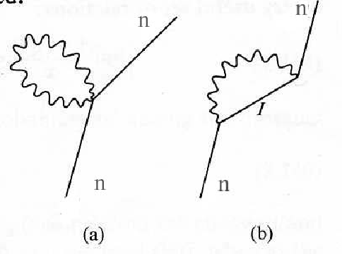
We can calculate the lowest order self energy corrections represented by the two Feynman diagrams below.
 term in second order time dependent perturbation theory.
A calculation of the first diagram will give the same result for a free electron and a bound electron,
while the second diagram will give different results because the intermediate states are different
if an electron is bound than they are if it is free.
We will therefore compute the amplitude from the second diagram.
term in second order time dependent perturbation theory.
A calculation of the first diagram will give the same result for a free electron and a bound electron,
while the second diagram will give different results because the intermediate states are different
if an electron is bound than they are if it is free.
We will therefore compute the amplitude from the second diagram.
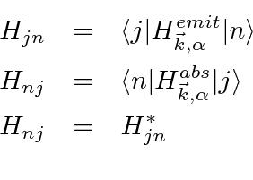
 specifying the photon emitted or absorbed leaving a reminder in the sum.
Recall from earlier calculations that the creation and annihilation operators just give a factor of 1
when a photon is emitted or absorbed.
specifying the photon emitted or absorbed leaving a reminder in the sum.
Recall from earlier calculations that the creation and annihilation operators just give a factor of 1
when a photon is emitted or absorbed.
From time dependent perturbation theory, the rate of change of the amplitude to be in a state is given by
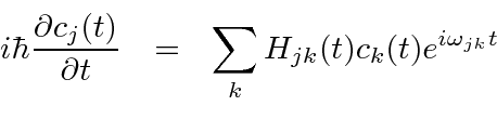
The differential equations for the amplitudes are then.
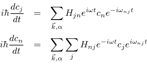
Our task is to solve these coupled equations. Previously, we did this by integration, but needed the assumption that the amplitude to be in the initial state was 1.
Since we are attempting to calculate an energy shift, let us make that assumption and plug it into the equations to verify the solution.
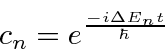
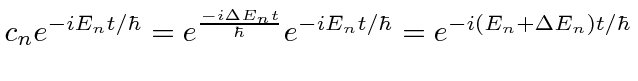
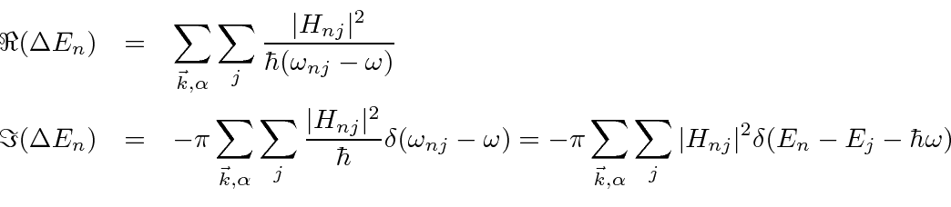
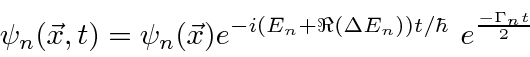
 will be a complex number, the real part of which represents an energy shift,
and the imaginary part of which represents the lifetime (and energy width) of the state.
will be a complex number, the real part of which represents an energy shift,
and the imaginary part of which represents the lifetime (and energy width) of the state.
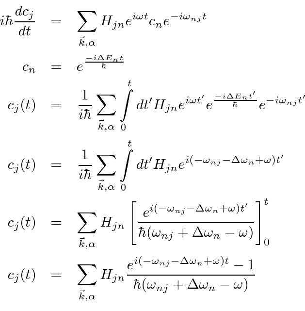
Substitute this back into the differential equation for
![]() to verify the solution
and to find out what
to verify the solution
and to find out what  is.
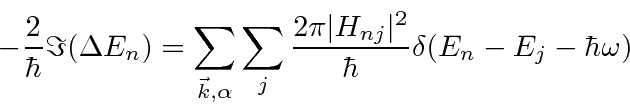
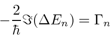
Note that the double sum over photons reduces to a single sum because we must absorb the same type of photon that was emitted.
(We have not explicitly carried along the photon state for economy.)
is.
Note that the double sum over photons reduces to a single sum because we must absorb the same type of photon that was emitted.
(We have not explicitly carried along the photon state for economy.)
 s from the right hand side of this equation.
We have something of the form
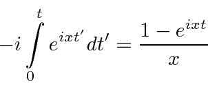
 , the function goes to zero at infinity.
In the lower half plane it blows up at infinity and on the axis, its not well defined.
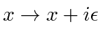
We will calculate our result in the upper half plane and take the limit as we approach the real axis.
, the function goes to zero at infinity.
In the lower half plane it blows up at infinity and on the axis, its not well defined.
We will calculate our result in the upper half plane and take the limit as we approach the real axis.
![\begin{eqnarray*}
\lim_{t\rightarrow\infty}{1-e^{ixt}\over x}=-\lim_{\epsilon\ri...
...[{x\over x^2+\epsilon^2}-{i\epsilon\over x^2+\epsilon^2}\right]
\end{eqnarray*}](img4113.png)
 there.
A little further analysis could show that the second term is a delta function.
there.
A little further analysis could show that the second term is a delta function.
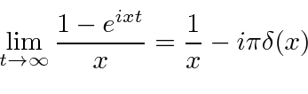
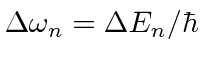
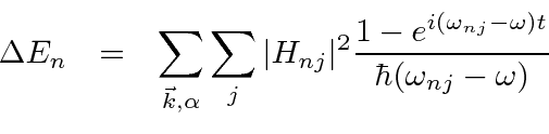
Recalling that
 ,
the real part of
corresponds to an energy shift in the state
,
the real part of
corresponds to an energy shift in the state
![]() and the imaginary part corresponds to a width.
and the imaginary part corresponds to a width.
 .
.
 .
It is valid up to about 2000 eV so we wish to cut off the calculation around there.
While this calculation clearly diverges, things are less clear here because of the eventually rapid oscillation of the
.
It is valid up to about 2000 eV so we wish to cut off the calculation around there.
While this calculation clearly diverges, things are less clear here because of the eventually rapid oscillation of the
It is the difference between the bound electron's self energy and that for a free electron in which we are interested.
Therefore, we will start with the free electron with a definite momentum
![]() .
The normalized wave function for the free electron is
.
The normalized wave function for the free electron is
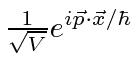 .
.
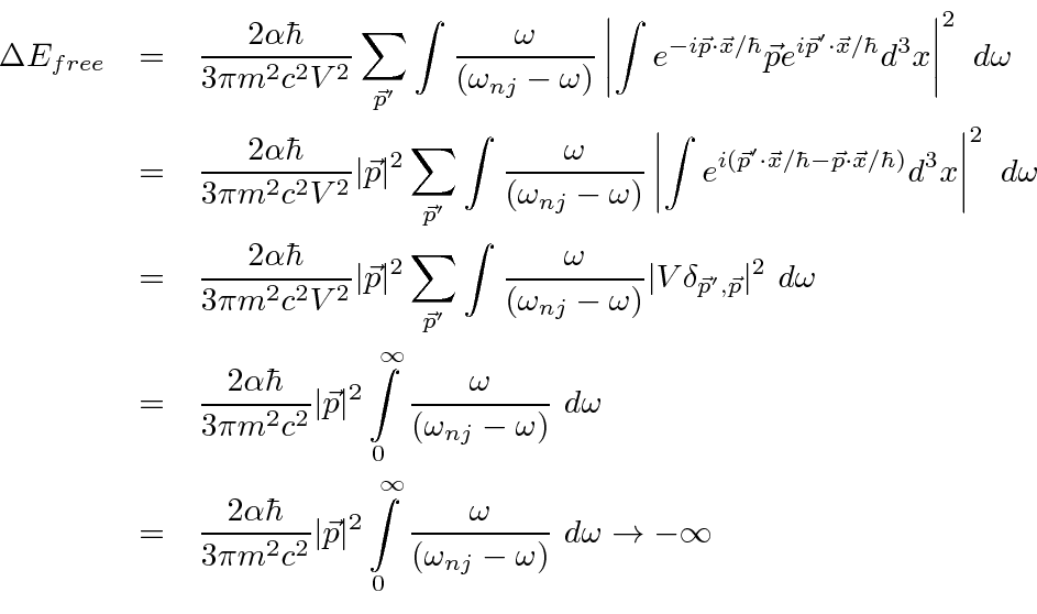
 .
For the E1 approximation, it should be
.
For the E1 approximation, it should be
 .
We will approximate
.
We will approximate
 since the integral is just giving us a number and
we are not interested in high accuracy here.
We will be more interested in accuracy in the next section when we compute the difference between free electron and bound electron
self energy corrections.
since the integral is just giving us a number and
we are not interested in high accuracy here.
We will be more interested in accuracy in the next section when we compute the difference between free electron and bound electron
self energy corrections.
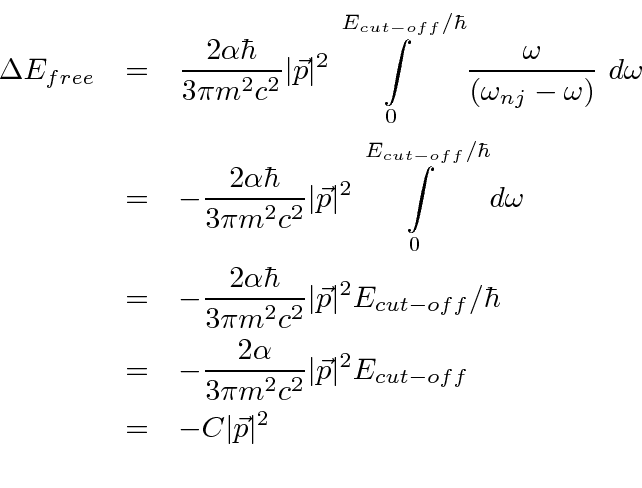
For a non-relativistic free electron the energy
 decreases as the mass of the electron increases,
so the negative sign corresponds to a positive shift in the electron's mass,
and hence an increase in the real energy of the electron.
Later, we will think of this as a renormalization of the electron's mass.
The electron starts off with some bare mass.
The self-energy due to the interaction of the electron's charge with its own radiation field
increases the mass to what is observed.
decreases as the mass of the electron increases,
so the negative sign corresponds to a positive shift in the electron's mass,
and hence an increase in the real energy of the electron.
Later, we will think of this as a renormalization of the electron's mass.
The electron starts off with some bare mass.
The self-energy due to the interaction of the electron's charge with its own radiation field
increases the mass to what is observed.
Note that the correction to the energy is a
constant times ![]() , like the non-relativistic formula for the kinetic energy.
, like the non-relativistic formula for the kinetic energy.
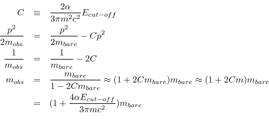
 , the correction to the mass is only about 0.3%,
but if we don't cut off, its infinite.
It makes no sense to trust our non-relativistic calculation up to infinite energy,
so we must proceed with the cut-off integral.
, the correction to the mass is only about 0.3%,
but if we don't cut off, its infinite.
It makes no sense to trust our non-relativistic calculation up to infinite energy,
so we must proceed with the cut-off integral.
If we use the Dirac theory, then we will be justified to move the cut-off up to very high energy. It turns out that the relativistic correction diverges logarithmically (instead of linearly) and the difference between bound and free electrons is finite relativistically (while it diverges logarithmically for our non-relativistic calculation).
Note that the self-energy of the free electron depends on the momentum of the electron,
so we cannot simply subtract it from our bound state calculation.
(What
![]() would we choose?)
Rather me must account for the mass renormalization.
We used the observed electron mass in the calculation of the Hydrogen bound state energies.
In so doing, we have already included some of the self energy correction and we must not double correct.
This is the subtraction we must make.
would we choose?)
Rather me must account for the mass renormalization.
We used the observed electron mass in the calculation of the Hydrogen bound state energies.
In so doing, we have already included some of the self energy correction and we must not double correct.
This is the subtraction we must make.
Its hard to keep all the minus signs straight in this calculation, particularly if we consider the bound and
continuum electron states separately.
The free particle correction to the electron mass is positive.
Because we ignore the rest energy of the electron in our non-relativistic calculations,
This makes a negative energy correction to both the bound (
 ) and
continuum (
) and
continuum (
 ).
Bound states and continuum states have the same fractional change in the energy.
We need to add back in a positive term in
to avoid double counting of the self-energy correction.
Since the bound state and continuum state terms have the same fractional change,
it is convenient to just use
for all the corrections.
).
Bound states and continuum states have the same fractional change in the energy.
We need to add back in a positive term in
to avoid double counting of the self-energy correction.
Since the bound state and continuum state terms have the same fractional change,
it is convenient to just use
for all the corrections.