Fourier Decomposition of Radiation Oscillators

Our goal is to write the Hamiltonian for the radiation field in terms of a sum of harmonic oscillator Hamiltonians. The first step is to write the radiation field in as simple a way as possible, as a sum of harmonic components. 
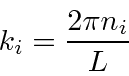
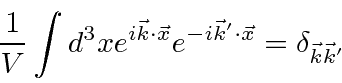
We will work in a cubic volume \bgroup\color{black}$V=L^3$\egroup and apply periodic boundary conditions on our electromagnetic waves. We also assume for now that there are no sources inside the region so that we can make a gauge transformation to make \bgroup\color{black}$A_0=0$\egroup and hence \bgroup\color{black}$\vec{\nabla}\cdot\vec{A}=0$\egroup. 
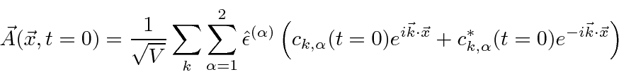
We decompose the field into its Fourier components at \bgroup\color{black}$t=0$\egroup

\begin{displaymath}\bgroup\color{black} \vec{A}(\vec{x},t=0)={1\over\sqrt{V}}\su...
...x}}+c_{k,\alpha}^*(t=0)e^{-i\vec{k}\cdot\vec{x}}\right) \egroup\end{displaymath}

where \bgroup\color{black}$\hat{\epsilon}^{(\alpha)}$\egroup are real unit vectors, and \bgroup\color{black}$c_{k,\alpha}$\egroup is the coefficient of the wave with wave vector \bgroup\color{black}$\vec{k}$\egroup and polarization vector \bgroup\color{black}$\hat{\epsilon}^{(\alpha)}$\egroup. Once the wave vector is chosen, the two polarization vectors must be picked so that \bgroup\color{black}$\hat{\epsilon}^{(1)}$\egroup, \bgroup\color{black}$\hat{\epsilon}^{(2)}$\egroup, and \bgroup\color{black}$\vec{k}$\egroup form a right handed orthogonal system. The components of the wave vector must satisfy

\begin{displaymath}\bgroup\color{black} k_i={2\pi n_i\over L} \egroup\end{displaymath}

due to the periodic boundary conditions. The factor out front is set to normalize the states nicely since

\begin{displaymath}\bgroup\color{black} {1\over V}\int d^3x e^{i\vec{k}\cdot\vec{x}} e^{-i\vec{k}'\cdot\vec{x}}=\delta_{\vec{k}\vec{k}'} \egroup\end{displaymath}

and

\begin{displaymath}\bgroup\color{black} \hat{\epsilon}^{(\alpha)}\cdot\hat{\epsilon}^{(\alpha')}=\delta_{\alpha\alpha'}. \egroup\end{displaymath}

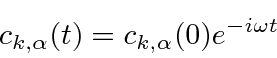
We know the time dependence of the waves from Maxwell's equation,

\begin{displaymath}\bgroup\color{black} c_{k,\alpha}(t)=c_{k,\alpha}(0)e^{-i\omega t} \egroup\end{displaymath}

where \bgroup\color{black}$\omega=kc$\egroup. We can now write the vector potential as a function of position and time.

\begin{displaymath}\bgroup\color{black} \vec{A}(\vec{x},t)={1\over\sqrt{V}}\sum\...
...c{x}}+c_{k,\alpha}^*(t)e^{-i\vec{k}\cdot\vec{x}}\right) \egroup\end{displaymath}

We may write this solution in several different ways, and use the best one for the calculation being performed. One nice way to write this is in terms 4-vector \bgroup\color{black}$k_\mu$\egroup, the wave number,

\begin{displaymath}\bgroup\color{black} k_\mu={p_\mu\over \hbar}=(k_x,k_y,k_z,ik)=(k_x,k_y,k_z,i{\omega\over c}) \egroup\end{displaymath}

so that

\begin{displaymath}\bgroup\color{black}k_\rho x_\rho=k\cdot x=\vec{k}\cdot\vec{x}-\omega t. \egroup\end{displaymath}

We can then write the radiation field in a more covariant way.

\begin{displaymath}\bgroup\color{black} \vec{A}(\vec{x},t)={1\over\sqrt{V}}\sum\...
...rho x_\rho}+c_{k,\alpha}^*(0)e^{-ik_\rho x_\rho}\right) \egroup\end{displaymath}

A convenient shorthand for calculations is possible by noticing that the second term is just the complex conjugate of the first.

\begin{displaymath}\bgroup\color{black} \vec{A}(\vec{x},t)={1\over\sqrt{V}}\sum\...
...}
\left(c_{k,\alpha}(0)e^{ik_\rho x_\rho}+ c.c. \right) \egroup\end{displaymath}


\begin{displaymath}\bgroup\color{black} \vec{A}(\vec{x},t)={1\over\sqrt{V}}\sum\...
...lon}^{(\alpha)}
c_{k,\alpha}(0)e^{ik_\rho x_\rho}+ c.c. \egroup\end{displaymath}

Note again that we have made this a transverse field by construction.
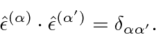
 The unit vectors \bgroup\color{black}$\hat{\epsilon}^{(\alpha)}$\egroup are transverse to the direction of propagation. Also note that we are working in a gauge with \bgroup\color{black}$A_4=0$\egroup
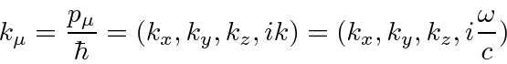
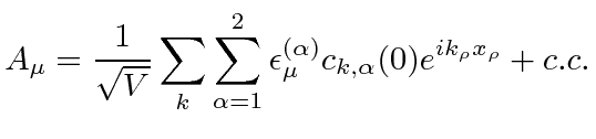
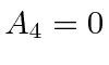
, so this can also represent the 4-vector form of the potential. 
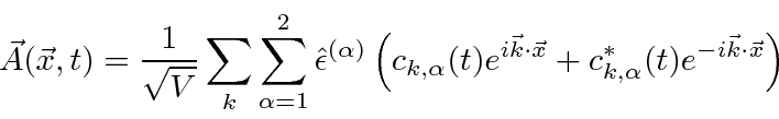
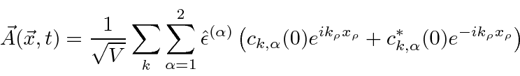
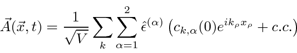
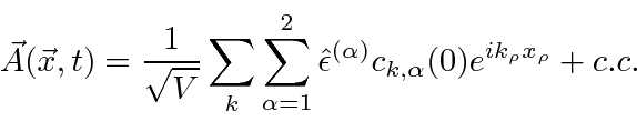
The Fourier decomposition of the radiation field can be written very simply.

\bgroup\color{black}$\displaystyle A_\mu ={1\over\sqrt{V}}\sum\limits_k\sum\limi...
...pha=1}^2\epsilon_\mu^{(\alpha)}
c_{k,\alpha}(0)e^{ik_\rho x_\rho}+ c.c. $\egroup
This choice of gauge makes switching between 4-vector and 3-vector expressions for the potential trivial.

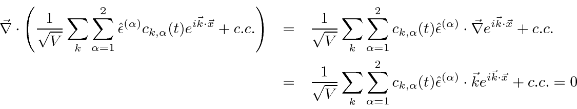
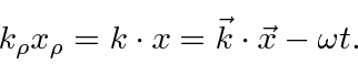
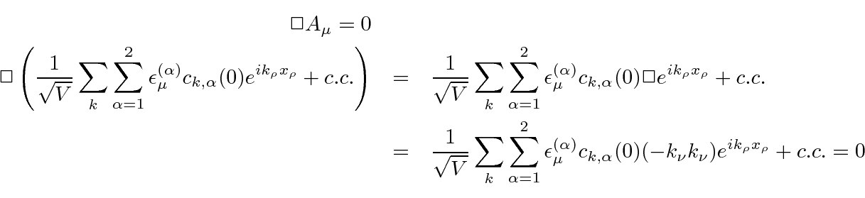
Let's verify that this decomposition of the radiation field satisfies the Maxwell equation, just for some practice. Its most convenient to use the covariant form of the equation and field.

\begin{eqnarray*}
\Box A_\mu=0 \\
\Box\left({1\over\sqrt{V}}\sum\limits_k\sum\l...
...a)}
c_{k,\alpha}(0)(-k_\nu k_\nu) e^{ik_\rho x_\rho}+ c.c.=0 \\
\end{eqnarray*}


The result is zero since \bgroup\color{black}$k_\nu k_\nu=k^2-k^2=0$\egroup.

Let's also verify that $\vec{\nabla}\cdot\vec{A}=0$.

\begin{eqnarray*}
\vec{\nabla}\cdot\left({1\over\sqrt{V}}\sum\limits_k\sum\limit...
...\epsilon}^{(\alpha)}\cdot\vec{k}e^{i\vec{k}\cdot\vec{x}}+ c.c.=0
\end{eqnarray*}


The result here is zero because \bgroup\color{black}$\hat{\epsilon}^{(\alpha)}\cdot\vec{k}=0$\egroup.

Jim Branson 2013-04-22