Quantization of the EM Field

The Hamiltonian for the Maxwell field may be used to quantize the field in much the same way that one dimensional wave mechanics was quantized. The radiation field can be shown to be the transverse part of the field $\vec{A}_\perp$ while static charges give rise to $A_\parallel$ and $A_0$.

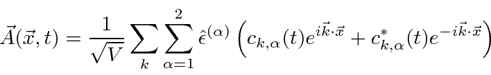
We decompose the radiation field into its Fourier components

$$\bgroup\color{black} \vec{A}(\vec{x},t)={1\over\sqrt{V}}\sum\... ...c{x}}+c_{k,\alpha}^*(t)e^{-i\vec{k}\cdot\vec{x}}\right) \egroup$$

where $\hat{\epsilon}^{(\alpha)}$ are real unit vectors, and $c_{k,\alpha}$ is the coefficient of the wave with wave vector $\vec{k}$ and polarization vector $\hat{\epsilon}^{(\alpha)}$. Once the wave vector is chosen, the two polarization vectors must be picked so that $\hat{\epsilon}^{(1)}$, $\hat{\epsilon}^{(2)}$, and $\vec{k}$ form a right handed orthogonal system.

Plugging the Fourier decomposition into the formula for the Hamiltonian density and using the transverse nature of the radiation field, we can compute the Hamiltonian (density integrated over volume).

$$\begin{eqnarray*} H&=&\sum\limits_{k,\alpha}\left({\omega\over c}\right)^2 \left... ...(t)c_{k,\alpha}^*(t)+c_{k,\alpha}^*(t)c_{k,\alpha}(t)\right] \\ \end{eqnarray*}$$

This Hamiltonian will be used to quantize the EM field. In calculating the Hamiltonian, care has been taken not to commute the Fourier coefficients and their conjugates.

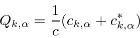
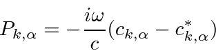
The canonical coordinate and momenta may be found

$$\bgroup\color{black} Q_{k,\alpha}={1\over c}(c_{k,\alpha}+c_{k,\alpha}^*) \egroup$$

$$\bgroup\color{black} P_{k,\alpha}=-{i\omega\over c}(c_{k,\alpha}-c_{k,\alpha}^*) \egroup$$

for the harmonic oscillator at each frequency. We assume that a coordinate and its conjugate momentum have the same commutator as in wave mechanics and that coordinates from different oscillators commute.

$$\begin{eqnarray*} \left[Q_{k,\alpha},P_{k',\alpha'}\right]&=&i\hbar\delta_{kk'}\... ...\right]&=&0 \\ \left[P_{k,\alpha},P_{k',\alpha'}\right]&=&0 \\ \end{eqnarray*}$$

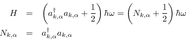
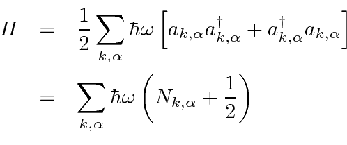
As was done for the 1D harmonic oscillator, we write the Hamiltonian in terms of raising and lowering operators that have the same commutation relations as in the 1D harmonic oscillator.

$$\begin{eqnarray*} a_{k,\alpha}&=&{1\over\sqrt{2\hbar\omega}}(\omega Q_{k,\alpha}... ...\alpha'}^\dagger\right]&=&\delta_{kk'}\delta_{\alpha\alpha'} \\ \end{eqnarray*}$$

This means everything we know about the raising and lowering operators applies here. Energies are in steps of $\hbar\omega$ and there must be a ground state. The states can be labeled by a quantum number $n_{k,\alpha}$.

$$\begin{eqnarray*} H&=&\left(a_{k,\alpha}^\dagger a_{k,\alpha}+{1\over 2}\right)\... ...r\omega \\ N_{k,\alpha}&=&a_{k,\alpha}^\dagger a_{k,\alpha} \\ \end{eqnarray*}$$

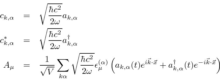
The Fourier coefficients can now be written in terms of the raising and lowering operators for the field.

$$\begin{eqnarray*} c_{k,\alpha}&=&\sqrt{\hbar c^2\over 2\omega}a_{k,\alpha} \\ c... ...{x}}+a_{k,\alpha}^\dagger(t)e^{-i\vec{k}\cdot\vec{x}}\right) \\ \end{eqnarray*}$$

$$\begin{eqnarray*} H&=&{1\over 2}\sum\limits_{k,\alpha}\hbar\omega\left[a_{k,\alp... ...ts_{k,\alpha}\hbar\omega\left(N_{k,\alpha}+{1\over 2}\right) \\ \end{eqnarray*}$$

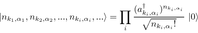
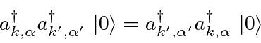
States of the field are given by the occupation number of each possible photon state.

$$\bgroup\color{black} \vert n_{k_1,\alpha_1},n_{k_2,\alpha_2},... ...,\alpha_i}}\over\sqrt{n_{k_i,\alpha_i}!}} \vert\rangle \egroup$$

Any state can be constructed by operating with creation operators on the vacuum state. Any state with multiple photons will automatically be symmetric under the interchange of pairs of photons because the operators commute.

$$\bgroup\color{black} a_{k,\alpha}^\dagger a_{k',\alpha'}^\dag... ...{k',\alpha'}^\dagger a_{k,\alpha}^\dagger \vert\rangle \egroup$$

This is essentially the same result as our earlier guess to put an $n+1$ in the emission operator.

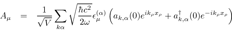
We can now write the quantized radiation field in terms of the operators at $t=0$.

$$\begin{eqnarray*} A_\mu &=&{1\over\sqrt{V}}\sum\limits_{k\alpha}\sqrt{\hbar c^2\... ...ho x_\rho}+a_{k,\alpha}^\dagger(0)e^{-ik_\rho x_\rho}\right) \\ \end{eqnarray*}$$

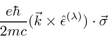
Beyond the Electric Dipole approximation, the next term in the expansion of $e^{i\vec{k}\cdot\vec{x}}$ is $i\vec{k}\cdot\vec{x}$. This term gets split according to its rotation and Lorentz transformation properties into the Electric Quadrupole term and the Magnetic Dipole term. The interaction of the electron spin with the magnetic field is of the same order and should be included together with the E2 and M1 terms.

$$\bgroup\color{black} {e\hbar\over 2mc} (\vec{k}\times\hat{\epsilon}^{(\lambda)})\cdot\vec{\sigma} \egroup$$

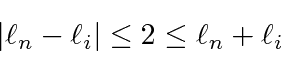
The Electric Quadrupole (E2) term does not change parity and gives us the selection rule.

$$\bgroup\color{black} \vert\ell_n-\ell_i\vert\leq 2\leq \ell_n+\ell_i \egroup$$

The Magnetic Dipole term (M1) does not change parity but may change the spin. Since it is an (axial) vector operator, it changes angular momentum by 0, +1, or -1 unit.

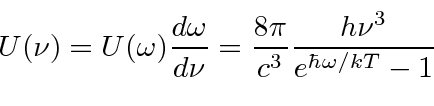
The quantized field is very helpful in the derivation of Plank's black body radiation formula that started the quantum revolution. By balancing the reaction rates proportional to $N$ and $N+1$ for absorption and emission in equilibrium the energy density in the radiation field inside a cavity is easily derived.

$$\begin{eqnarray*} U(\nu)=U(\omega){d\omega\over d\nu}= {8\pi\over c^3}{h\nu^3\over e^{\hbar\omega/kT}-1} \\ \end{eqnarray*}$$