Next: Decay Rates for the Up: Radiation in Atoms Previous: Radiation in Atoms Contents
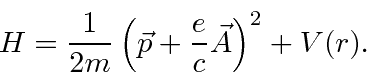
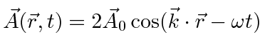
Lets assume that there is some ElectroMagnetic field around the atom.
The field is not extremely strong so that the
![]() term can be neglected (for our purposes)
and we will work in the Coulomb gauge for which
term can be neglected (for our purposes)
and we will work in the Coulomb gauge for which
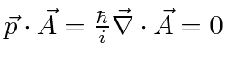 .
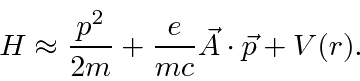
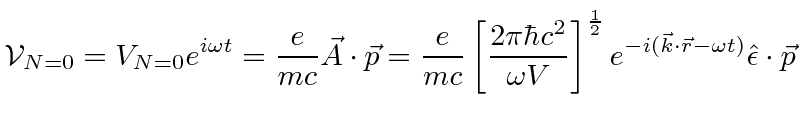
The Hamiltonian then becomes
.
The Hamiltonian then becomes
Lets also assume that the field has some frequency
![]() and corresponding wave vector
and corresponding wave vector
![]() .
(In fact, and arbitrary field would be a linear combination of many frequencies, directions of propagation, and polarizations.)
.
(In fact, and arbitrary field would be a linear combination of many frequencies, directions of propagation, and polarizations.)

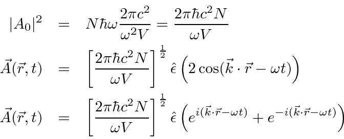
We need to quantize the EM field into photons satisfying Plank's original hypothesis,
![]() .
Lets start by writing
.
Lets start by writing
![]() in terms of the number of photons in the field
(at frequency
in terms of the number of photons in the field
(at frequency
![]() and wave vector
and wave vector
![]() ).
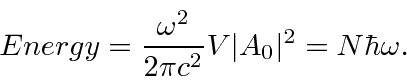
Using
classical E&M to compute the energy in a field
represented by a vector potential
).
Using
classical E&M to compute the energy in a field
represented by a vector potential
 ,
we find that the energy inside a volume
,
we find that the energy inside a volume
![]() is
is
But what about decays of atoms with no applied field?
Here we need to go beyond our classical E&M calculation and quantize the field.
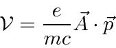
Since the terms in the perturbation above emit or absorb a photon, and the photon has energy
![]() ,
lets assume the number of photons in the field is the
,
lets assume the number of photons in the field is the ![]() of a harmonic oscillator.
It has the right steps in energy.
Essentially, we are postulating that the vacuum contains an infinite number of harmonic oscillators,
one for each wave vector (or frequency...) of light.
of a harmonic oscillator.
It has the right steps in energy.
Essentially, we are postulating that the vacuum contains an infinite number of harmonic oscillators,
one for each wave vector (or frequency...) of light.
We now want to go from a classical harmonic oscillator to a quantum oscillator, in which the ground state
energy is not zero, and the hence the perturbing field is never really zero.
We do this by
changing ![]() to
to  in the term that creates a photon in analogy to the raising operator
![]() in the HO.
With this change, our perturbation becomes
in the HO.
With this change, our perturbation becomes
![\begin{eqnarray*}
\vec{A}(\vec{r},t)&=&\left[{2\pi\hbar c^2\over\omega V}\right]...
...\omega t)}+\sqrt{N+1}e^{-i(\vec{k}\cdot\vec{r}-\omega t)}\right)
\end{eqnarray*}](img398.png)
Now there is a perturbation even with no applied field (
![]() ).
).
 |
We have taken a step toward quantization of the EM field, at least when we emit or absorb a photon. With this step, we can correctly compute the EM transition rates in atoms. Note that we have postulated that the vacuum has an infinite number of oscillators corresponding to the different possible modes of EM waves. When we quantize these oscillators, the vacuum has a ground state energy density in the EM field (equivalent to half a photon of each type). That vacuum EM field is then responsible for the spontaneous decay of excited states of atoms through the emission of a photon. We have not yet written the quantum equations that the EM field must satisfy, although they are closely related to Maxwell's equations.
Jim Branson 2013-04-22