Simple Mechanical Systems and Fields

This section is a review of mechanical systems largely from the point of view of Lagrangian dynamics. In particular, we review the equations of a string as an example of a field theory in one dimension.

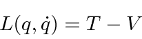
We start with the Lagrangian of a discrete system like a single particle.

\begin{displaymath}\bgroup\color{black} L(q,\dot{q})=T-V \egroup\end{displaymath}

Lagrange's equations are

\begin{displaymath}\bgroup\color{black}{d \over dt}\left({\partial L\over\partial\dot{q}_i}\right)-{\partial L\over\partial q_i}=0 \egroup\end{displaymath}

where the \bgroup\color{black}$q_i$\egroup are the coordinates of the particle. This equation is derivable from the principle of least action.

\begin{displaymath}\bgroup\color{black} \delta \int\limits_{t_1}^{t_2}L(q_i,\dot{q}_i)dt=0 \egroup\end{displaymath}

Similarly, we can define the Hamiltonian

\begin{displaymath}\bgroup\color{black} H(q_i,p_i)=\sum\limits_ip_i\dot{q}_i-L \egroup\end{displaymath}

where \bgroup\color{black}$p_i$\egroup are the momenta conjugate to the coordinates \bgroup\color{black}$q_i$\egroup.

\begin{displaymath}\bgroup\color{black} p_i={\partial L\over\partial\dot{q}_i} \egroup\end{displaymath}

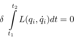
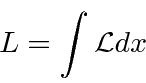
For a continuous system, like a string, the Lagrangian is an integral of a Lagrangian density function.
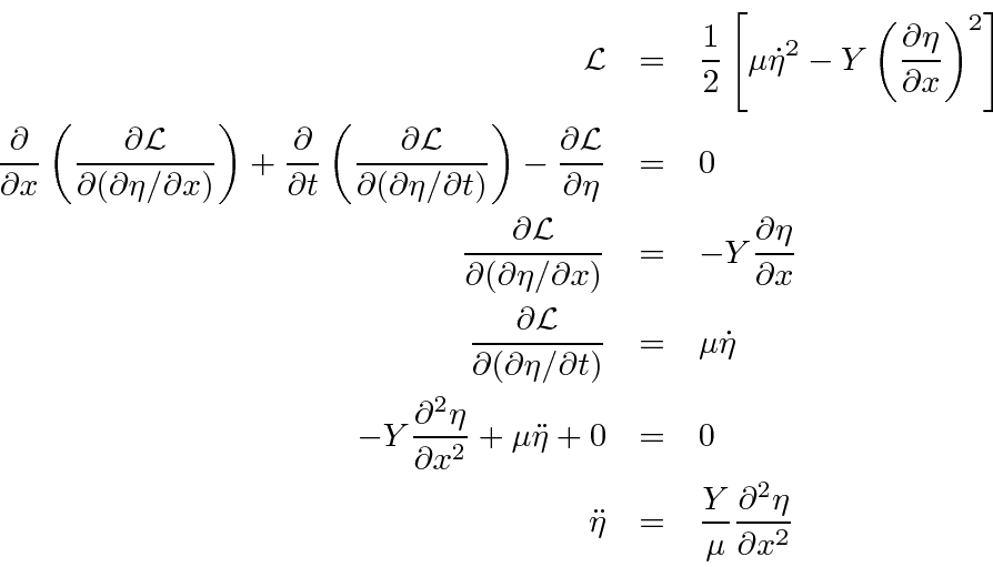
\begin{displaymath}\bgroup\color{black} L=\int {\cal L} dx \egroup\end{displaymath}

For example, for a string,

\begin{displaymath}\bgroup\color{black} {\cal L}={1\over 2}\left[\mu\dot{\eta}^2-Y\left({\partial\eta\over\partial x}\right)^2\right] \egroup\end{displaymath}

where \bgroup\color{black}$Y$\egroup is Young's modulus for the material of the string and \bgroup\color{black}$\mu$\egroup is the mass density. The Euler-Lagrange Equation for a continuous system is also derivable from the principle of least action states above. For the string, this would be.

\begin{displaymath}\bgroup\color{black} {\partial\over\partial x}\left({\partial...
...rtial t)}\right)
-{\partial{\cal L}\over\partial\eta}=0 \egroup\end{displaymath}

Recall that the Lagrangian is a function of \bgroup\color{black}$\eta$\egroup and its space and time derivatives.

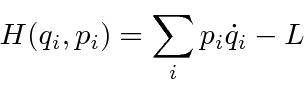
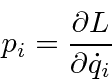
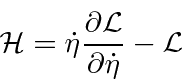
The Hamiltonian density can be computed from the Lagrangian density and is a function of the coordinate \bgroup\color{black}$\eta$\egroup and its conjugate momentum.

\begin{displaymath}\bgroup\color{black} {\cal H}=\dot{\eta}{\partial{\cal L}\over\partial\dot{\eta}}-{\cal L} \egroup\end{displaymath}

In this example of a string, \bgroup\color{black}$\eta(x,t)$\egroup is a simple scalar field. The string has a displacement at each point along it which varies as a function of time.

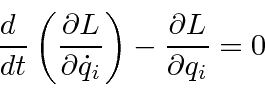
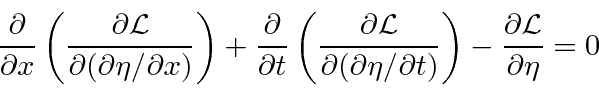
If we apply the Euler-Lagrange equation, we get a differential equation that the string's displacement will satisfy.

\begin{eqnarray*}
{\cal L}&=&{1\over 2}\left[\mu\dot{\eta}^2-Y\left({\partial\et...
...0 \\
\ddot{\eta}&=&{Y\over\mu}{\partial^2\eta\over\partial x^2}
\end{eqnarray*}


This is the wave equation for the string. There are easier ways to get to this wave equation, but, as we move away from simple mechanical systems, a formal way of proceeding will be very helpful.

Jim Branson 2013-04-22