Next: Thomson Scattering Up: Dirac Equation Previous: The Expected Velocity and Contents
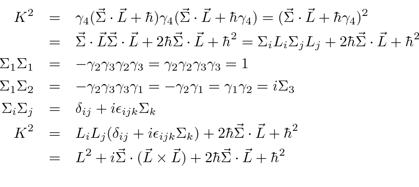
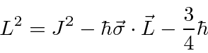
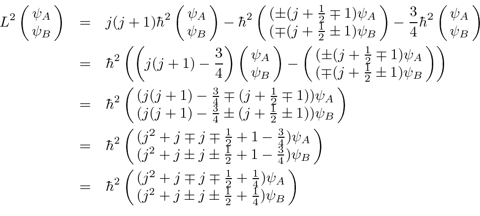
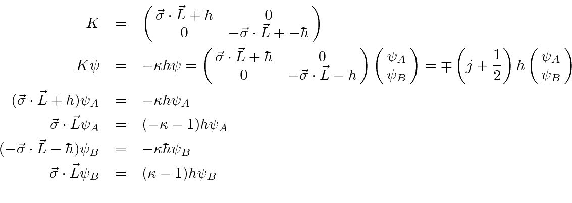
We have shown in the section on conserved quantities that the operator
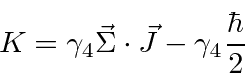
The operator ![]() may be written in several ways.
may be written in several ways.
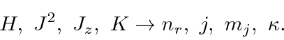
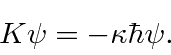
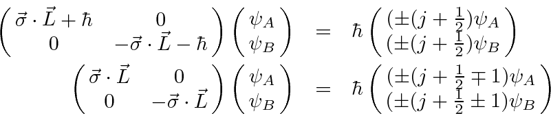
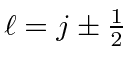
Assume that the eigenvalues of ![]() are given by
are given by
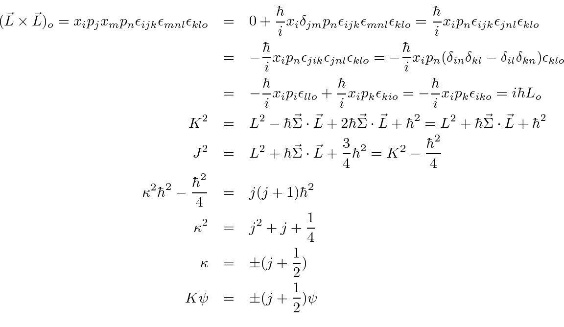
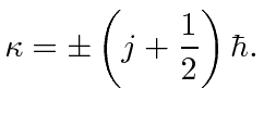
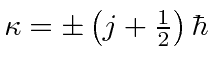
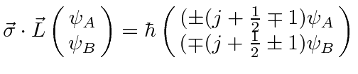
The eigenvalues of
![]() are
are
 |
 .
.

 are eigenstates of
 |
 from NR QM.
We simply check that it is the same here.
from NR QM.
We simply check that it is the same here.
 are eigenstates of
|
 |
 |
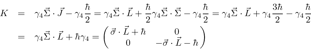
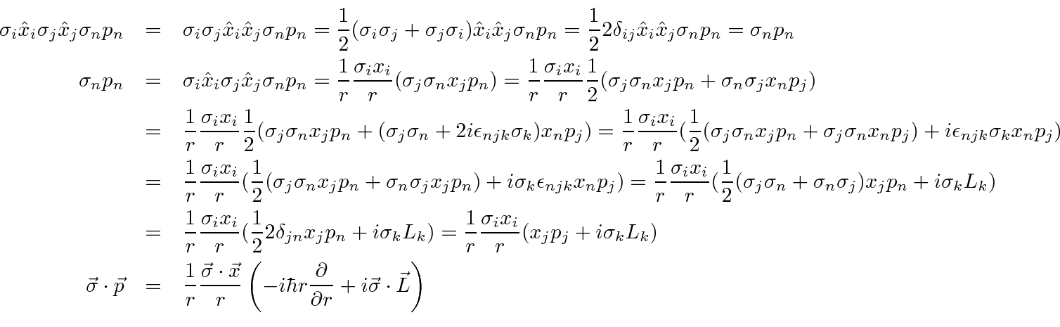
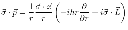
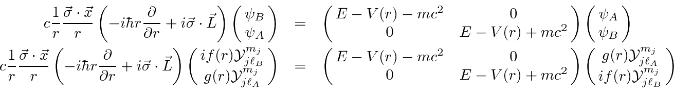
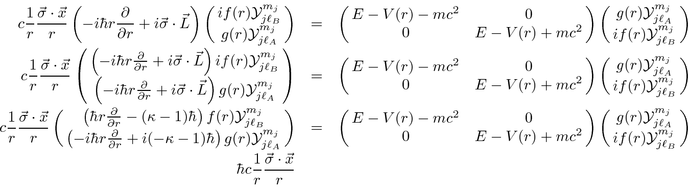
We can use commutation and anticommutation relations to write
 in terms of separate angular and radial operators.
 |
Note that the operators
 and
and
![]() act only on the angular momentum parts of the state.
There are no radial derivatives so they commute with
act only on the angular momentum parts of the state.
There are no radial derivatives so they commute with
 .
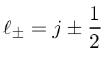
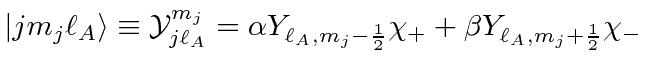
Lets pick a shorthand notation for the angular momentum eigenstates we must use.
These have quantum numbers
.
Lets pick a shorthand notation for the angular momentum eigenstates we must use.
These have quantum numbers
![]() ,
,
![]() , and
, and
![]() .
.
![]() will have
will have
 and
must have the other possible value of
and
must have the other possible value of
![]() which we label
which we label
![]() .
Following the notation of Sakurai, we will call the state
.
Following the notation of Sakurai, we will call the state
 .
(Note that our previous functions made use of
.
(Note that our previous functions made use of
 particularly in the calculation of
![]() and
and
![]() .)
.)
The effect of the two operators related to angular momentum can be deduced.
First,
![]() is related to
is related to
![]() .
For positive
.
For positive
![]() ,
,
![]() has
has
 .
For negative
.
For negative
![]() ,
,
![]() has
has
 .
For either,
has the opposite relation for
.
For either,
has the opposite relation for
![]() , indicating why the full spinor is not an eigenstate of
, indicating why the full spinor is not an eigenstate of
![]() .
.
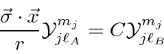
 is a pseudoscalar operator.
It therefore changes parity and the parity of the state is given by
is a pseudoscalar operator.
It therefore changes parity and the parity of the state is given by
 ; so it must change
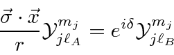
 is one, as is clear from the derivation above,
so we know the effect of this operator up to a phase factor.
is one, as is clear from the derivation above,
so we know the effect of this operator up to a phase factor.
 .
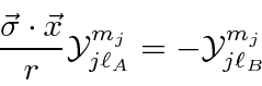
For our conventions, the factor is
.
For our conventions, the factor is
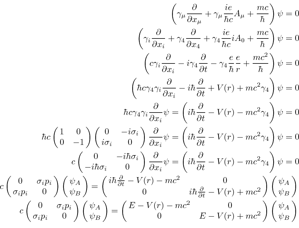
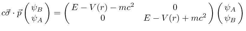
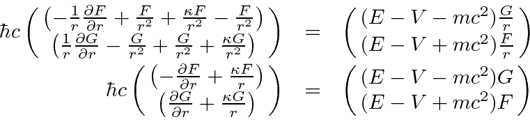
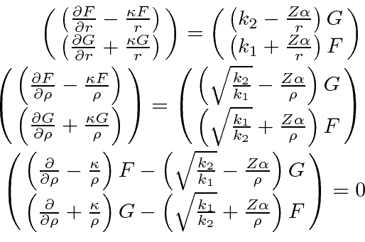
We now have everything we need to get to the radial equations.
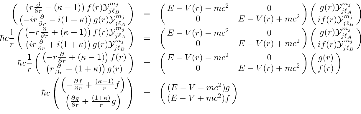
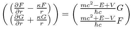
This is now a set of two coupled radial equations.
We can simplify them a bit by making the substitutions
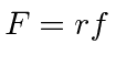 and
and
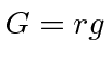 .
The extra term from the derivative cancels the 1's that are with
.
The extra term from the derivative cancels the 1's that are with
![]() s.
s.
 |
These equations are true for any spherically symmetric potential.
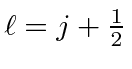
Now it is time to specialize to the hydrogen atom for which
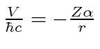 .
We define
.
We define
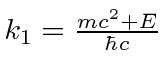 and
and
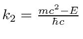 and the dimensionless
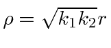 .
The equations then become.
.
The equations then become.
With the guidance of the non-relativistic solutions, we will postulate a solution of the form
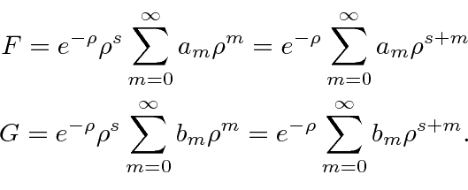
 if we pick the right
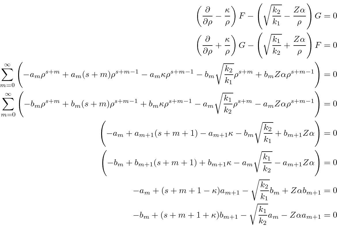
|
 |
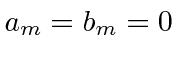
For the lowest order term
![]() , we need to have a solution without lower powers.
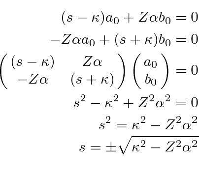
This means that we look at the
, we need to have a solution without lower powers.
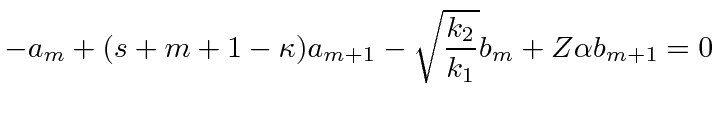
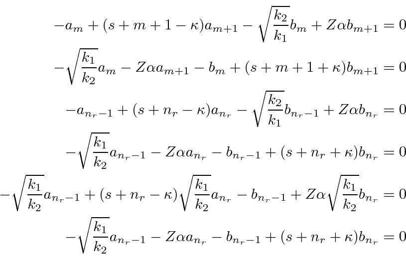
This means that we look at the  recursion relations with
 and solve the equations.
As usual, the series must terminate at some  for the state to normalizable.
This can be seen approximately by assuming either the
for the state to normalizable.
This can be seen approximately by assuming either the
![]() 's or the
's or the
![]() 's are small and noting that the series is that of a positive exponential.
's are small and noting that the series is that of a positive exponential.
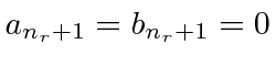
Assume the series for
![]() and
and
![]() terminate at the same
terminate at the same ![]() .
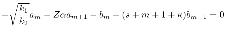
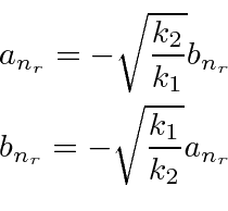
We can then take the equations in the coefficients and set
.
We can then take the equations in the coefficients and set
 to get relationships between
 and
and
 .
.
The final step is to use this result in the recursion relations for 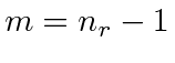 to
find a condition on
to
find a condition on ![]() which must be satisfied for the series to terminate.
Note that this choice of
which must be satisfied for the series to terminate.
Note that this choice of
![]() connects
and
to the rest of the series giving nontrivial conditions on
connects
and
to the rest of the series giving nontrivial conditions on
![]() .
We already have the information from the next step in the recursion which gives
.
.
We already have the information from the next step in the recursion which gives
.
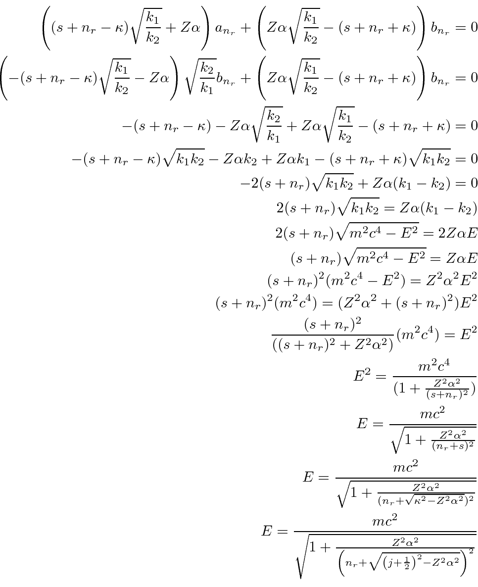
Using the quantum numbers from four mutually commuting operators, we have solved the radial equation in a similar way as for the non-relativistic case yielding the exact energy relation for relativistic Quantum Mechanics.
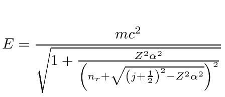 |
We can identify the standard principle quantum number in this case as
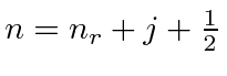 .
This result gives the same answer as our non-relativistic calculation to order
.
This result gives the same answer as our non-relativistic calculation to order
![]() but is also
correct to higher order.
It is an exact solution to the quantum mechanics problem posed but does not include the effects of
field theory, such as the Lamb shift and the anomalous magnetic moment of the electron.
but is also
correct to higher order.
It is an exact solution to the quantum mechanics problem posed but does not include the effects of
field theory, such as the Lamb shift and the anomalous magnetic moment of the electron.
Relativistic corrections become quite important for high
![]() atoms in which the typical velocity of electrons
in the most inner shells is of order
atoms in which the typical velocity of electrons
in the most inner shells is of order
![]() .
.
Jim Branson 2013-04-22