Next: Dirac Equation Up: Electron Self Energy Corrections Previous: Electron Self Energy Corrections Contents
 and
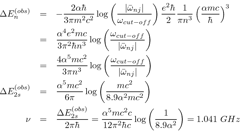
and  states in Hydrogen
to have a frequency of 1.06 GHz, (a wavelength of about 30 cm).
(The shift is now accurately measured to be 1057.864 MHz.)
This is about the same size as the hyperfine splitting of the ground state.
states in Hydrogen
to have a frequency of 1.06 GHz, (a wavelength of about 30 cm).
(The shift is now accurately measured to be 1057.864 MHz.)
This is about the same size as the hyperfine splitting of the ground state.

The technique used was quite interesting.
They made a beam of Hydrogen atoms in the state, which has a very long lifetime because of selection rules.
Microwave radiation with a (fixed) frequency of 2395 MHz was used to cause transitions to the
 state
and a magnetic field was adjusted to shift the energy of the states until the rate was largest.
The decay of the
state
and a magnetic field was adjusted to shift the energy of the states until the rate was largest.
The decay of the  state to the ground state was observed to determine the transition rate.
From this, they were able to deduce the shift between the
state to the ground state was observed to determine the transition rate.
From this, they were able to deduce the shift between the
 and
and
 states.
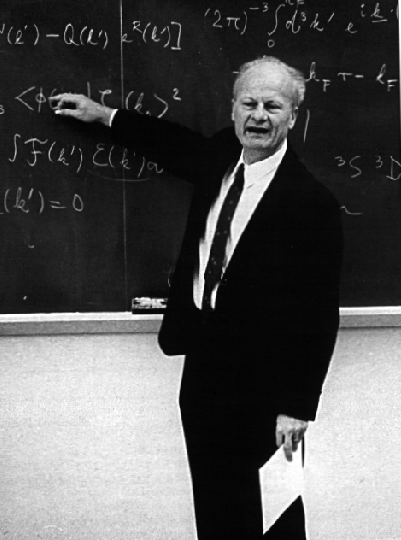
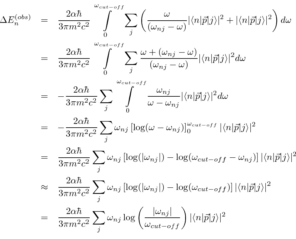
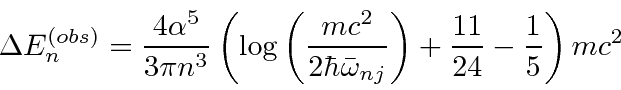
Hans Bethe used non-relativistic quantum mechanics to calculate the self-energy correction to account for this observation.
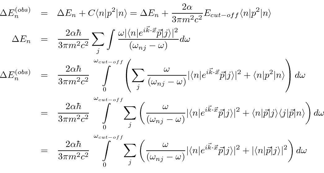
It is now necessary to discuss approximations needed to complete this calculation.
In particular, the electric dipole approximation will be of great help, however, it is certainly not warranted for
large photon energies.
For a good E1 approximation we need
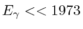 eV.
On the other hand, we want the cut-off for the calculation to be of order
eV.
On the other hand, we want the cut-off for the calculation to be of order
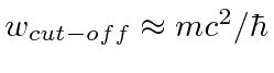 .
We will use the E1 approximation and the high cut-off, as Bethe did, to get the right answer.
At the end, the result from a relativistic calculation can be tacked on to show why it turns out to be the right answer.
(We aren't aiming for the worlds best calculation anyway.)
.
We will use the E1 approximation and the high cut-off, as Bethe did, to get the right answer.
At the end, the result from a relativistic calculation can be tacked on to show why it turns out to be the right answer.
(We aren't aiming for the worlds best calculation anyway.)
 is
is
 using a typical clever quantum mechanics calculation.
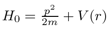
The basic Hamiltonian for the Hydrogen atom is
using a typical clever quantum mechanics calculation.
The basic Hamiltonian for the Hydrogen atom is
 .
.
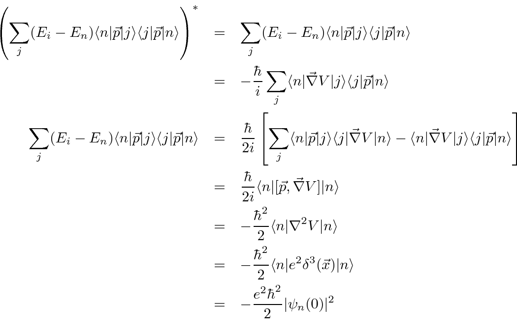
![\begin{eqnarray*}[\vec{p},H_0]&=&[\vec{p},V]={\hbar\over i}\vec{\nabla}V \\
\la...
...ec{p}\vert j\rangle\langle j\vert\vec{\nabla}V\vert n\rangle \\
\end{eqnarray*}](img4147.png)
 and
and
 .
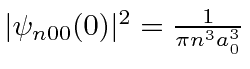
Therefore, only the s states will shift in energy appreciably.
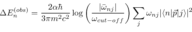
The shift will be.
.
Therefore, only the s states will shift in energy appreciably.
The shift will be.
 yields.
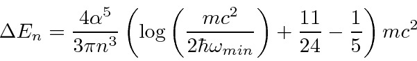
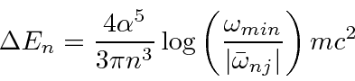
 cancels.
In this calculation, the
cancels.
In this calculation, the
The Lamb shift splits the and states which are otherwise degenerate.
Its origin is purely from field theory.
The experimental measurement of the Lamb shift stimulated theorists to develop Quantum ElectroDynamics.
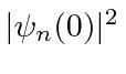
The correction increases the energy of s states.
One may think of the physical origin as the electron becoming less pointlike as virtual photons are emitted and reabsorbed.
Spreading the electron out a bit decreases the effect of being in the deepest part of the potential,
right at the origin.
Based on the energy shift,
I estimate that the electron in the 2s state is spread out by about 0.005 Angstroms,
much more than the size of the nucleus.
The anomalous magnetic moment of the electron,
 , which can also be calculated in field theory,
makes a small contribution to the Lamb shift.
, which can also be calculated in field theory,
makes a small contribution to the Lamb shift.