Next: Classical Maxwell Fields Up: Classical Scalar Fields Previous: Simple Mechanical Systems and Contents
Assume we have a field defined everywhere in space and time.
For simplicity we will start with a scalar field(instead of the vector... fields of E&M).

The Euler-Lagrange equation derived from the principle of least action is
Since we are aiming for a description of relativistic quantum mechanics,
it will benefit us to write our equations in a covariant way.
I think this also simplifies the equations.
We will follow the notation of Sakurai.
(The convention does not really matter and one should not get hung up on it.)
As usual the Latin indices like
 will run from 1 to 3 and represent the space coordinates.
The Greek indices like
will run from 1 to 3 and represent the space coordinates.
The Greek indices like
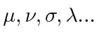 will run from 1 to 4.
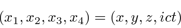
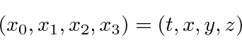
Sakurai would give the spacetime coordinate vector either as
will run from 1 to 4.
Sakurai would give the spacetime coordinate vector either as
We will not use the so called covariant and contravariant indices.
Instead we will put an
![]() on the fourth component of a vector which give that component a
on the fourth component of a vector which give that component a
![]() sign
in a dot product.
sign
in a dot product.
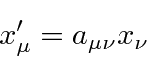
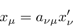
The spacetime coordinate
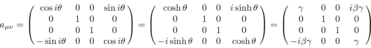
![]() is a Lorentz vector transforming under rotations and boosts as follows.
is a Lorentz vector transforming under rotations and boosts as follows.
 are real while the
 and
and
 are imaginary in our convention.
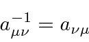
Thus we may compute the coordinate using the inverse transformation.
are imaginary in our convention.
Thus we may compute the coordinate using the inverse transformation.
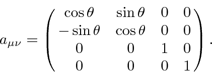
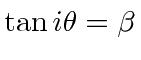
The Lorentz transformation matrix to a coordinate system boosted along the x direction is.
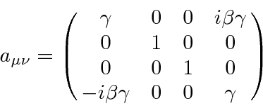
 .
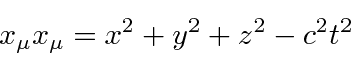
Since we are in Minkowski space where we need a minus sign on the time component of dot products, we need to add an
.
Since we are in Minkowski space where we need a minus sign on the time component of dot products, we need to add an
 .
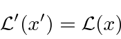
We will make essentially no use of Lorentz transformations because we will write our theories in terms of Lorentz scalarswhenever possible.
For example, our Lagrangian density should be invariant.
.
We will make essentially no use of Lorentz transformations because we will write our theories in terms of Lorentz scalarswhenever possible.
For example, our Lagrangian density should be invariant.
 .
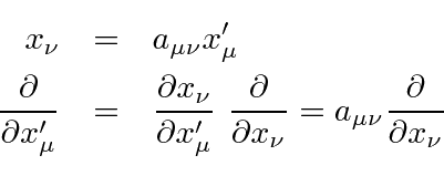
We need to know what the transformation properties of this are.
We can compute this from the transformations and the chain rule.
.
We need to know what the transformation properties of this are.
We can compute this from the transformations and the chain rule.
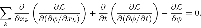
With this, lets work on the Euler-Lagrange equation to get it into covariant shape.
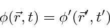
Remember that the field
![]() is a Lorentz scalar.
is a Lorentz scalar.
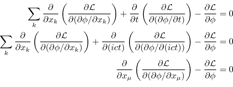
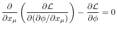
This is the Euler-Lagrange equation for a single scalar field.
Each term in this equation is a Lorentz scalar, if
![]() is a scalar.
is a scalar.
 |
Now we want to find a reasonable Lagrangian for a scalar field.
The Lagrangian depends on the
![]() and its derivatives.
It should not depend explicitly on the coordinates
and its derivatives.
It should not depend explicitly on the coordinates
![]() , since that would violate translation
and/or rotation invariance.
We also want to come out with a linear wave equation so that high powers of the field should not appear.
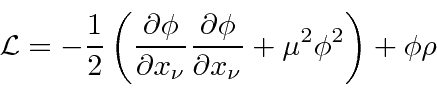
The only Lagrangian we can choose (up to unimportant constants) is
, since that would violate translation
and/or rotation invariance.
We also want to come out with a linear wave equation so that high powers of the field should not appear.
The only Lagrangian we can choose (up to unimportant constants) is
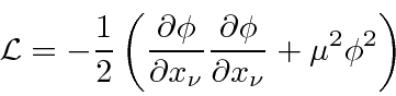
 definition.
Remember that
definition.
Remember that
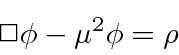
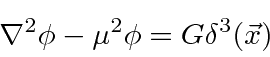
With this Lagrangian, the Euler-Lagrange equation is.
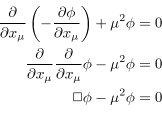
This is the known as the Klein-Gordon equation.
It is a good relativistic equation for a massive scalar field.
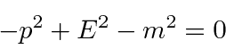
It was also an early candidate for the relativistic equivalent of the Schrödinger equation for electrons
because it basically has the relativistic analog of the energy relation inherent in the Schrödinger equation.
Writing that relation in the order terms appear in the Klein-Gordon equation above we get (letting
![]() briefly).
briefly).
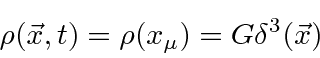
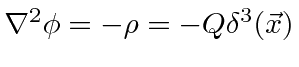
So far we have the Lagrangian and wave equation for a ``free'' scalar field.
There are no sources of the field (the equivalent of charges and currents in electromagnetism.)
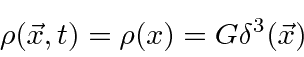
Lets assume the source density is
 .
The source term must be a scalar function so,
we add the term
.
The source term must be a scalar function so,
we add the term
![]() to the Lagrangian.
to the Lagrangian.
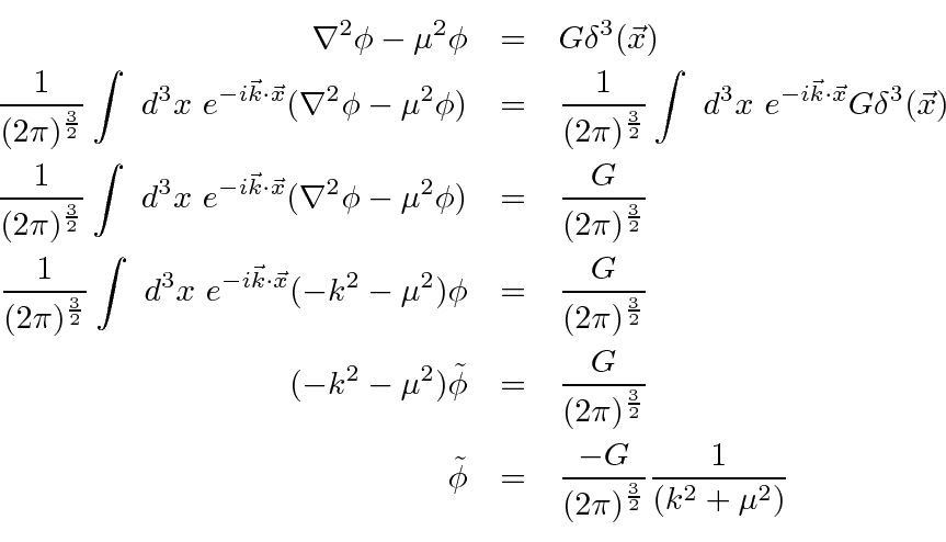
Any source density can be built up from point sources so it is useful to understand the
field generated by a point source as we do for electromagnetism.

 ,
,
 .
This is a field that falls off much faster than
.
This is a field that falls off much faster than
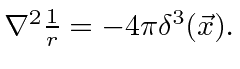
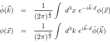
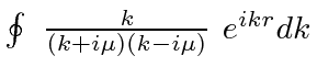
Now we solve for the scalar field from a point source by Fourier transforming the wave equation. Define the Fourier transforms to be.
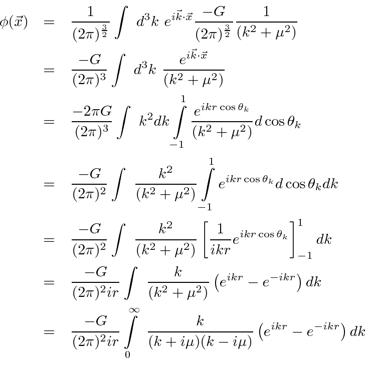
We now have the Fourier transform of the field of a point source. If we can transform back to position space, we will have the field. This is a fairly standard type of problem in quantum mechanics.
If the integrand is a function of the complex variable
![]() ,
a pole is of the form
,
a pole is of the form
![]() where
where
![]() is called the residue at the pole.
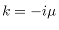
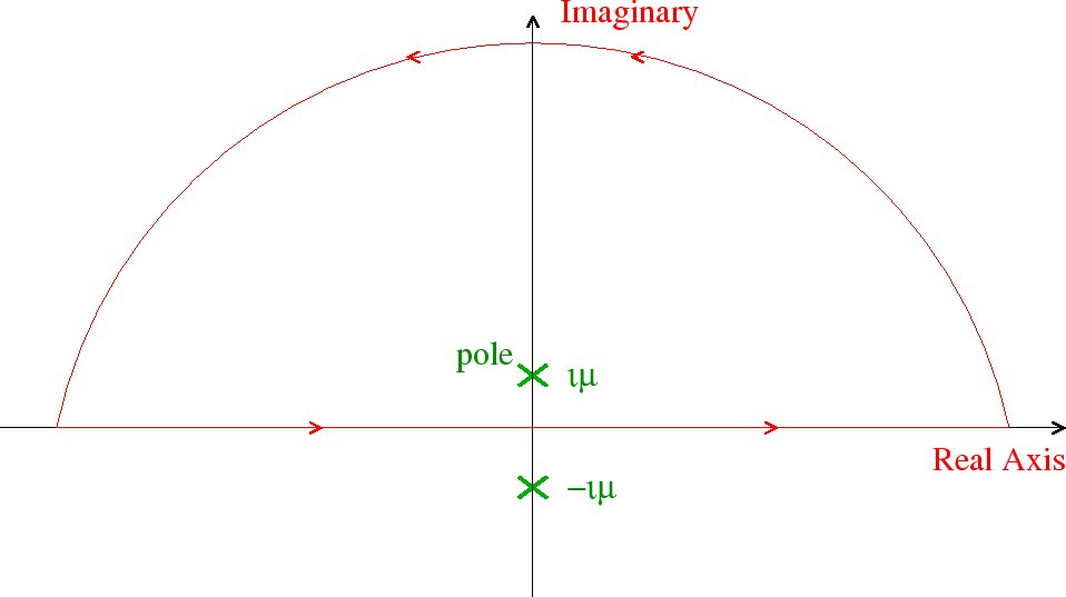
The integrand above has two poles, one at
is called the residue at the pole.
The integrand above has two poles, one at
 and the other at
 .
The integral we are interested in is just along the real axis
so we want the integral along the rest of the contour to give zero.
That's easy to do since the integrand goes to zero at infinity on the real axis and
the exponentials go to zero either at positive or negative infinity for the imaginary part of
.
The integral we are interested in is just along the real axis
so we want the integral along the rest of the contour to give zero.
That's easy to do since the integrand goes to zero at infinity on the real axis and
the exponentials go to zero either at positive or negative infinity for the imaginary part of
![]() .
Examine the integral
.
Examine the integral
 around a contour in the upper half plane as shown below.
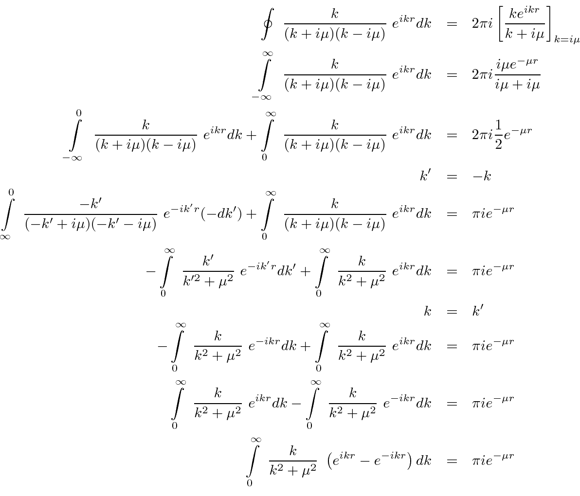
 .
The residue at the pole is
.
The residue at the pole is
![\begin{displaymath}\bgroup\color{black} \left[{ke^{ikr}\over k+i\mu}\right]_{k=i...
...={i\mu e^{-\mu r}\over i\mu+i\mu}={1\over 2}e^{-\mu r}. \egroup\end{displaymath}](img3818.png)
The integrand goes to zero exponentially on the semicircle at infinity so only the real axis contributes to the integral along the contour. The integral along the real axis can be manipulated to do the whole problem for us.
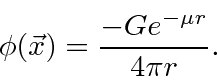
Plug the integral into the Fourier transform we were computing.
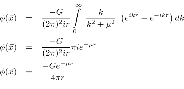
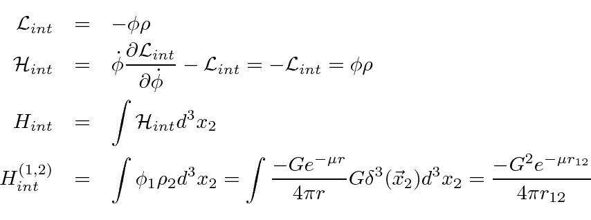
In this case, it is simple to compute the interaction Hamiltonian from the interaction Lagrangian
and the potential between two particles.
Lets assume we have two particles, each with the same interaction with the field.
This was proposed by Yukawa as the nuclear force. He predicted a scalar particle with a mass close to that of the pion before the pion was discovered. His prediction of the mass was based on the range of the nuclear force, on the order of one Fermi. In some sense, his prediction is approximately correct. Pion exchange can explain much of the nuclear force but does not explain all the details. Pions and nucleons have since been show to be composite particles with internal structure. Other composites with masses larger than the pion also play a role in the force between nucleons.
Pions were also found to come in three charges:
![]() ,
,
![]() , and
, and
![]() .
This would lead us to develop a complex scalar field as done in the text.
Its not our goal right now so we will skip this.
Its interesting to note that the Higgs Boson is also represented by a complex scalar field.
.
This would lead us to develop a complex scalar field as done in the text.
Its not our goal right now so we will skip this.
Its interesting to note that the Higgs Boson is also represented by a complex scalar field.
We have developed a covariant classical theory for a scalar field. The Lagrangian density is a Lorentz scalar function. We have included an interaction term to provide a source for the field. Now we will attempt to do the same for classical electromagnetism.