Next: Scattering from a Screened Up: Quantum Physics 130 Previous: Sample Test Problems Contents
This material is covered in Gasiorowicz Chapter 23.
Scattering of one object from another is perhaps our best way of observing and learning about the microscopic world. Indeed it is the scattering of light from objects and the subsequent detection of the scattered light with our eyes that gives us the best information about the macroscopic world. We can learn the shapes of objects as well as some color properties simply by observing scattered light.
There is a limit to what we can learn with visible light. In Quantum Mechanics we know that we cannot discern details of microscopic systems (like atoms) that are smaller than the wavelength of the particle we are scattering. Since the minimum wavelength of visible light is about 0.25 microns, we cannot see atoms or anything smaller even with the use of optical microscopes. The physics of atoms, nuclei, subatomic particles, and the fundamental particles and interactions in nature must be studied by scattering particles of higher energy than the photons of visible light.
Scattering is also something that we are familiar with from our every day experience. For example, billiard balls scatter from each other in a predictable way. We can fairly easily calculate how billiard balls would scatter if the collisions were elastic but with some energy loss and the possibility of transfer of energy to spin, the calculation becomes more difficult.
Let us take the macroscopic example of BBs scattering from billiard balls as an example to study.
We will motivate some of the terminology used in scattering macroscopically.
Assume we fire a BB at a billiard ball.
If we miss the BB does not scatter.
If we hit, the BB bounces off the ball and goes off in a direction different from the original direction.
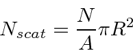
Assume our aim is bad and that the BB has a uniform probability distribution over the area around the billiard ball.
The area of the projection of the billiard ball into two dimensions is just
![]() if
if
![]() is the radius of the
billiard ball.
Assume the BB is much smaller so that its radius can be neglected for now.
is the radius of the
billiard ball.
Assume the BB is much smaller so that its radius can be neglected for now.
We can then say something about the probability for a scattering to occur if we know the area of the projection of the billiard ball
and number of BBs per unit area that we shot.
In normal scattering experiments, we have a beam of particles and
we know the number of particles per second.
We measure the number of scatters per second
so we just divide the above equation by the time period
![]() to get rates.
to get rates.

Clearly there is more information available from scattering than whether a particle scatters or not.
For example, Rutherford discovered that atomic nucleus by seeing that high energy alpha particles sometimes
backscatter from a foil containing atoms.
The atomic model of the time did not allow this since the positive charge was spread over a large volume.
We measure the probability to scatter into different directions.
This will also happen in the case of the BB and the billiard ball.
The polar angle of scattering will depend on the ``impact parameter'' of the incoming BB.
We can measure the scattering into some small solid angle
![]() .
The part of the cross section
.
The part of the cross section
![]() that scatters into that solid angle can be called
the differential cross section
that scatters into that solid angle can be called
the differential cross section
![]() .
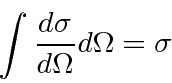
The integral over solid angle will give us back the total cross section.
.
The integral over solid angle will give us back the total cross section.
The idea of cross sections and incident fluxes translates well to the quantum mechanics we are using.
If the incoming beam is a plane wave, that is a beam of particles of definite momentum or wave number,
we can describe it simply in terms of the number or particles per unit area per second, the incident flux.
The scattered particle is also a plane wave going in the direction defined by
![]() .
What is left is the interaction between the target particle and the beam particle which causes the
transition from the initial plane wave state to the final plane wave state.
.
What is left is the interaction between the target particle and the beam particle which causes the
transition from the initial plane wave state to the final plane wave state.
We have already studied one approximation method for scattering called
a partial wave analysis.
It is good for scattering potentials of limited range and for low energy scattering.
It divides the incoming plane wave in to partial waves with definite angular momentum.
The high angular momentum components of the wave will not scatter (much) because they
are at large distance from the scattering potential where that potential is very small.
We may then deal with just the first few terms (or even just the
![]() term) in the expansion.
We showed that the incoming partial wave and the outgoing wave can differ only by a phase shift for elastic scattering.
If we calculate this phase shift
term) in the expansion.
We showed that the incoming partial wave and the outgoing wave can differ only by a phase shift for elastic scattering.
If we calculate this phase shift
![]() , we can then determine the differential scattering cross section.
, we can then determine the differential scattering cross section.
Let's review some of the equations.
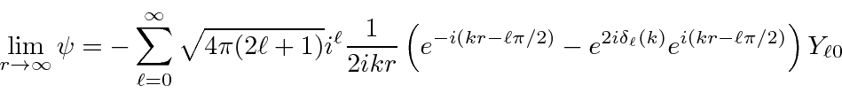
A plane wave can be decomposed into a sum of spherical waves with definite angular momenta
which goes to a simple sum of incoming and outgoing spherical waves at large
![]() .
.

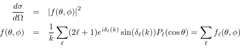
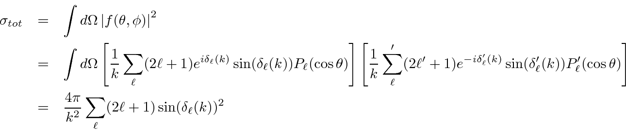
We can compute the differential cross section for elastic scattering.
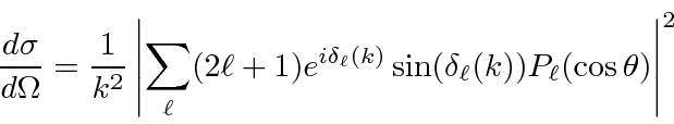
As an example, this has been used to
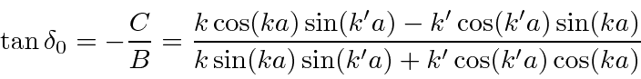
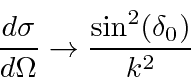
compute the cross section for scattering from a spherical potential well
assuming only the
![]() phase shift was significant.
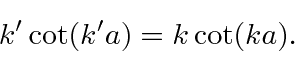
By matching the boundary conditions at the boundary of the spherical well, we determined the phase shift.
phase shift was significant.
By matching the boundary conditions at the boundary of the spherical well, we determined the phase shift.
We can compute the total scattering cross section using the relation
 .
.
 .
.
![\begin{eqnarray*}
f(\theta=0,\phi)&=&{1\over k}\sum\limits_\ell (2\ell +1)e^{i\d...
...
\sigma_{tot}&=&{4\pi\over k}Im\left[f(\theta=0,\phi)\right] \\
\end{eqnarray*}](img3723.png)
We have not treated inelastic scattering.
Inelastic scattering can be a complex and interesting process.
It was with high energy inelastic scattering of electrons from protons that the quark structure of the proton was ``seen''.
In fact, the electrons appeared to be scattering from essentially free quarks inside the proton.
The proton was broken up into sometimes many particles in the process but the data could be simply analyzed using the scatter electron.
In a phase shift analysis, inelastic scattering removes flux from the outgoing spherical waves.
 , with 0 represent complete absorption of the partial wave and 1 representing purely elastic scattering.
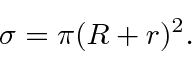
An interesting example of the effect of absorption (or inelastic production of another state) is the black disk.
The disk has a definite radius
, with 0 represent complete absorption of the partial wave and 1 representing purely elastic scattering.
An interesting example of the effect of absorption (or inelastic production of another state) is the black disk.
The disk has a definite radius
 .
If one works out this problem, one finds that there is an inelastic scattering cross section of
.
If one works out this problem, one finds that there is an inelastic scattering cross section of
 .
Somewhat surprisingly the total elastic scattering cross section is
.
Somewhat surprisingly the total elastic scattering cross section is
 .
The disk absorbs part of the beam and there is also diffraction around the sharp edges.
That is, the removal of the outgoing spherical partial waves modifies the plane wave to include scattered waves.
.
The disk absorbs part of the beam and there is also diffraction around the sharp edges.
That is, the removal of the outgoing spherical partial waves modifies the plane wave to include scattered waves.
For high energies relative to the inverse range of the potential, a partial wave analysis is not helpful and it is far better to use perturbation theory. The Born approximation is valid for high energy and weak potentials. If the potential is weak, only one or two terms in the perturbation series need be calculated.
If we work in the usual center of mass system, we have a problem with one particle scattering in a potential.
The incoming plane wave can be written as

The elastic scattering matrix element is

 .
We notice that this is just proportional to the Fourier Transform of the potential.
.
We notice that this is just proportional to the Fourier Transform of the potential.
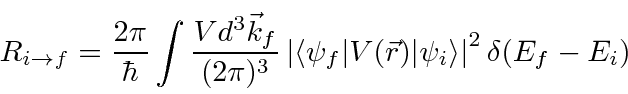
Assuming for now non-relativistic final state particles we calculate
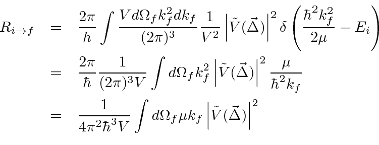
We now need to convert this transition rate to a cross section.
Our wave functions are normalize to one particle per unit volume and we should modify that so that there is a flux of one particle per square
centimeter per second to get a cross section.
To do this we set the volume to be
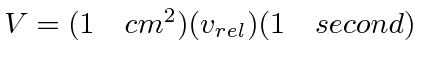 .
The relative velocity is just the momentum divided by the reduced mass.
.
The relative velocity is just the momentum divided by the reduced mass.
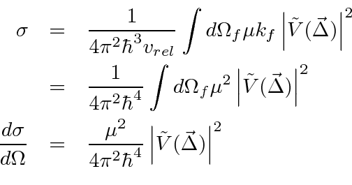
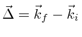
This is a very useful formula for scattering from a weak potential or for scattering at high energy for problems in which the
cross section gets small because the Fourier Transform of the potential diminishes for large values of
![]() .
It is not good for scattering due to the strong interaction since cross sections are large and do not typically decrease at high energy.
Note that the matrix elements and hence the scattering amplitudes calculated in the Born approximation are real
and therefore do not satisfy the Optical Theorem.
This is a shortcoming of the approximation.
.
It is not good for scattering due to the strong interaction since cross sections are large and do not typically decrease at high energy.
Note that the matrix elements and hence the scattering amplitudes calculated in the Born approximation are real
and therefore do not satisfy the Optical Theorem.
This is a shortcoming of the approximation.