Angular Distributions

We may also deduce the angular distribution of photons from our calculation. Lets take the 2p to 1s calculation as an example. We had the equation for the decay rate.

$$\bgroup\color{black} \Gamma_{tot}={\alpha\omega_{in}^3\over 2... ...ilon_y\over\sqrt{2}}Y_{1-1}\right)Y_{1m_i}\right\vert^2 \egroup$$

We have performed that radial integration which will be unchanged. Assume that we start in a polarized state with $m_i=1$. We then look at our result for the angular integration in the matrix element

$$\begin{eqnarray*} \left\vert\int d\Omega Y_{00}^* \left(\epsilon_zY_{10}+{-\epsi... ...ver 4\pi} \left({1\over 2}(\epsilon_x^2+\epsilon_y^2)\right) \\ \end{eqnarray*}$$

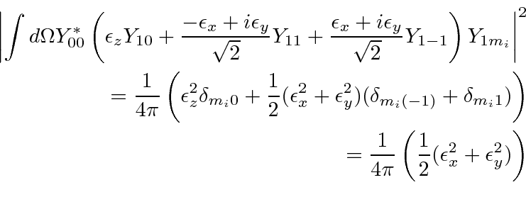where we have set $m_i=1$ eliminating two terms.

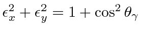
Lets study the rate as a function of the angle of the photon from the z axis, $\theta_\gamma$. The rate will be independent of the azimuthal angle. We see that the rate is proportional to $\epsilon_x^2+\epsilon_y^2$. We still must sum over the two independent transverse polarizations. For clarity, assume that $\phi=0$ and the photon is therefore emitted in the x-z plane. One transverse polarization can be in the y direction. The other is in the x-z plane perpendicular to the direction of the photon. The x component is proportional to $\cos\theta_\gamma$. So the rate is proportional to $\epsilon_x^2+\epsilon_y^2=1+\cos^2\theta_\gamma$.

If we assume that $m_i=0$ then only the $\epsilon_z$ term remains and the rate is proportional to $\epsilon_z^2$. The angular distribution then goes like $\sin^2\theta_\gamma$.