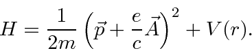
Next: Classical Field Theory Up: Course Summary Previous: Time Dependent Perturbation Theory Contents
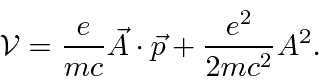
 term.
Both the decay of excited atomic states with the emission of radiation and the excitation of atoms
with the absorption of radiation can be calculated.
term.
Both the decay of excited atomic states with the emission of radiation and the excitation of atoms
with the absorption of radiation can be calculated.
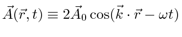
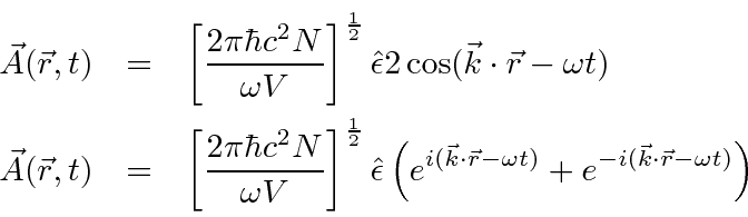
An arbitrary EM field can be Fourier analyzed to give a sum of components of definite frequency.
Consider the vector potential for one such component,
 .
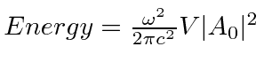
The energy in the field is
.
The energy in the field is
 .
If the field is quantized (as we will later show) with photons of energy
.
If the field is quantized (as we will later show) with photons of energy
![]() ,
we may write field strength in terms of the number of photons
,
we may write field strength in terms of the number of photons
![]() .
.
Think of the EM field as a harmonic oscillator at each frequency, the negative exponential corresponds to a raising operator
for the field and the positive exponential to a lowering operator.
In analogy to the quantum 1D harmonic oscillator we replace
 by
by
 in the raising operator case.
![\begin{eqnarray*}
\vec{A}(\vec{r},t)&=&\left[{2\pi\hbar c^2\over\omega V}\right]...
...\omega t)}+\sqrt{N+1}e^{-i(\vec{k}\cdot\vec{r}-\omega t)}\right)
\end{eqnarray*}](img398.png)
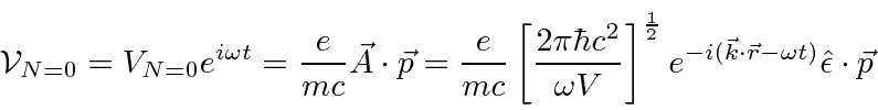
With this change, which will later be justified with the quantization of the field,
there is a perturbation even with no applied field (
![]() )
)
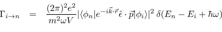
Plugging this
![]() field into the first order time dependent perturbation equations, the decay rate for an atomic
state can be computed.
field into the first order time dependent perturbation equations, the decay rate for an atomic
state can be computed.
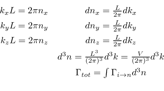
To get the total decay rate, we must sum over the allowed final states.
We can assume that the atom remains at rest as a very good approximation, but,
the final photon states must be carefully considered.
Applying periodic boundary conditions in a cubic volume
![]() ,
the integral over final states can be done as indicated below.
,
the integral over final states can be done as indicated below.
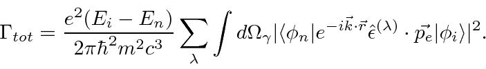
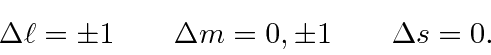
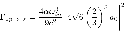
Computation of the atomic matrix element is usually done in the
Electric Dipole approximation
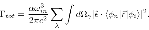

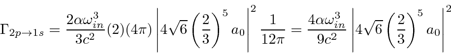
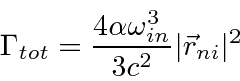
We derive a simple result for the total decay rate of a state, summed over final photon polarization
and integrated over photon direction.
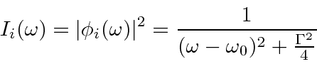
The total decay rate is related to the energy width of an excited state, as might be expected from the uncertainty principle.
The Full Width at Half Maximum (FWHM) of the energy distribution of a state is
 .
The distribution in frequency follows a Breit-Wigner distribution.
.
The distribution in frequency follows a Breit-Wigner distribution.
In addition to the inherent energy width of a state, other effects can influence measured widths, including collision broadening, Doppler broadening, and atomic recoil.
The quantum theory of EM radiation can be used to understand many phenomena, including photon angular distributions, photon polarization, LASERs, the Mössbauer effect, the photoelectric effect, the scattering of light, and x-ray absorption.