Next: Homework Problems Up: Derivations and Computations Previous: Derivations and Computations Contents
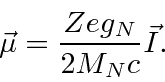


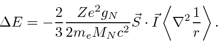
Then we compute the energy shift in first order perturbation theory for s states.

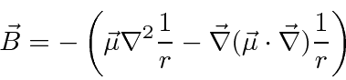
The second term can be simplified because of the spherical symmetry of s states.
(Basically the derivative with respect to x is odd in x so when the integral is done,
only the terms where
 are nonzero).
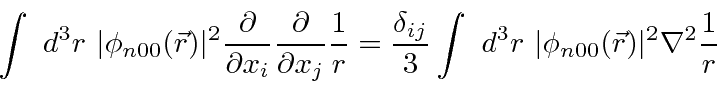
So we have
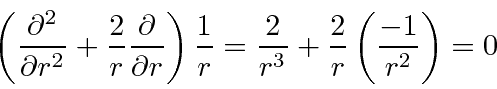
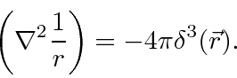
Now working out the
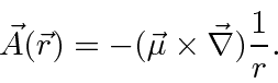
![]() term in spherical coordinates,
term in spherical coordinates,
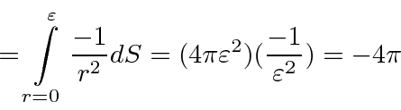
To find the effect at
![]() we will integrate.
we will integrate.
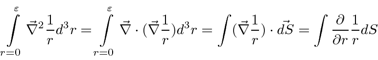
Simply writing the
![]() in terms of
in terms of
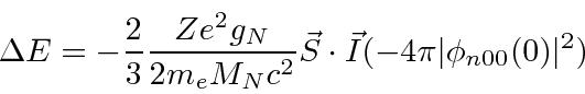
![]() and regrouping, we get
and regrouping, we get
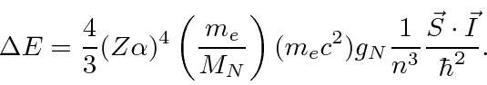
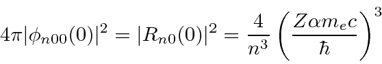
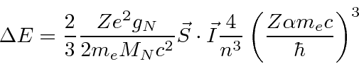
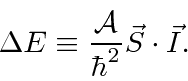
We will sometimes group the constants such that
(The textbook has numerous mistakes in this section.)