Next: Examples Up: Hyperfine Structure Previous: Hyperfine Splitting Contents
If we apply a B-field the states will split further.
As usual, we choose our coordinates so that the field is in
![]() direction.
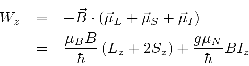
The perturbation then is
direction.
The perturbation then is
As an examples of perturbation theory, we will work this problem for weak fields,
for strong fields, and also work the general case for intermediate fields.
Just as in the Zeeman effect, if one perturbation is much bigger than another, we
choose the set of states in which the larger perturbation is diagonal.
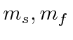
In this case, the hyperfine splitting is diagonal in states of definite
![]() while
the above perturbation due to the B field is diagonal in states of definite
while
the above perturbation due to the B field is diagonal in states of definite
![]() .
For a weak field, the hyperfine dominates and we use the states of definite
.
For a weak field, the hyperfine dominates and we use the states of definite
![]() .
For a strong field, we use the
.
For a strong field, we use the
 states.
If the two perturbations are of the same order, we must diagonalize the full
perturbation matrix.
This calculation will always be correct but more time consuming.
states.
If the two perturbations are of the same order, we must diagonalize the full
perturbation matrix.
This calculation will always be correct but more time consuming.
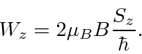
We can estimate the field at which the perturbations are the same size by
comparing
 to
to
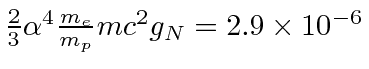 .
The weak field limit is achieved if
.
The weak field limit is achieved if
 gauss.
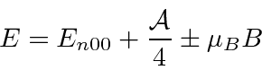
* Example:
The Hyperfine Splitting in a Weak B Field.*
The result of this is example is quite simple
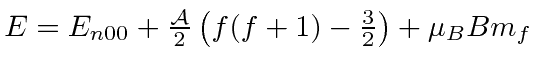 .
It has the hyperfine term we computed before and adds a term proportional to
.
It has the hyperfine term we computed before and adds a term proportional to
![]() which depends on
which depends on
 .
.
In the strong field limit we use states
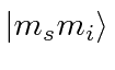 and treat the
hyperfine interaction as a perturbation.
The unperturbed energies of these states are
and treat the
hyperfine interaction as a perturbation.
The unperturbed energies of these states are
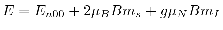 .
We kept the small term due to the nuclear moment in the B field without extra effort.
.
We kept the small term due to the nuclear moment in the B field without extra effort.
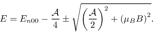
* Example:
The Hyperfine Splitting in a Strong B Field.*
The result in this case is

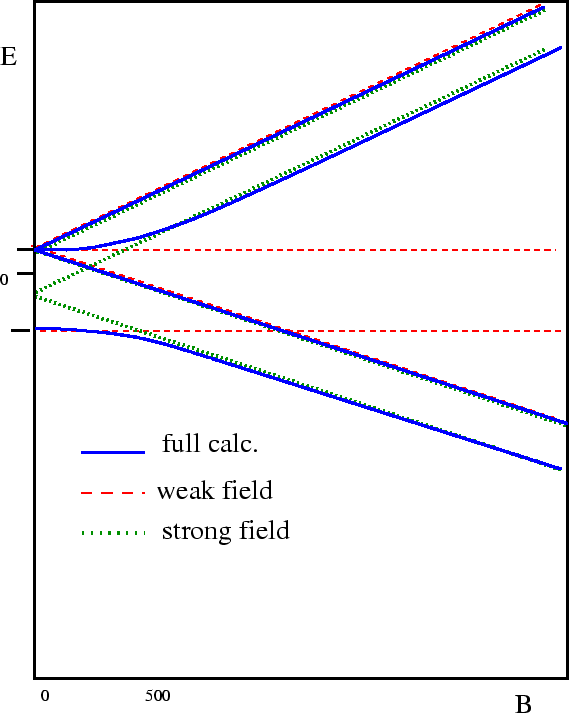
Finally, we do the full calculation.
* Example:
The Hyperfine Splitting in an Intermediate B Field.*
The general result consists of four energies which depend on the strength of the B field.
Two of the energy eigenstates mix in a way that also depends on B.
The four energies are
We can make a more general calculation, in which the interaction of the
nuclear magnetic moment is of the same order as the electron.
This occurs in muonic hydrogen or positronium.
* Example:
The Hyperfine Splitting in an Intermediate B Field.*
Jim Branson 2013-04-22