Review of the Classical Equations of Electricity and Magnetism in CGS Units
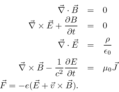
You may be most familiar with Maxwell's equations and the Lorentz force law in SI units as given below.
These equations have needless extra constants (not) of nature in them so we don't like to work in these units.
Since the Lorentz force law depends on the product of the charge and the field, there is the freedom to, for example,
increase the field by a factor of 2 but decrease the charge by a factor of 2 at the same time.
This will put a factor of 4 into Maxwell's equations but not change physics.
Similar tradeoffs can be made with the magnetic field strength and the constant on the Lorentz force law.
The choices made in CGS units are more physical (but still not perfect).
There are no extra constants other than
 .
Our textbook and many other advanced texts use CGS units and so will we in this chapter.
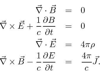
Maxwell's Equations in CGS units are
.
Our textbook and many other advanced texts use CGS units and so will we in this chapter.
Maxwell's Equations in CGS units are
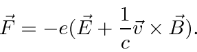
The Lorentz Force is
In fact, an even better definition (rationalized Heaviside-Lorentz units) of the charges and fields can be made
as shown in the introduction to field theory in chapter 32.
For now we will stick with the more standard CGS version of Maxwell's equations.
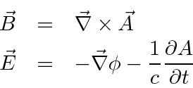
If we derive the fields from potentials,
then the first two Maxwell equations are automatically satisfied.
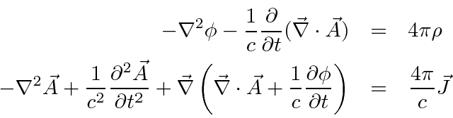
Applying the second two equations we get wave equations in the potentials.
These derivations
are fairly simple using Einstein notation.
The two results we want to use as inputs for our study of Quantum Physics are
- the classical gauge symmetry and
- the classical Hamiltonian.
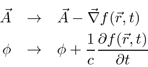
The Maxwell equations are invariant under a gauge transformation of the potentials.
Note that when we quantize the field, the potentials will play the role that wave functions
do for the electron, so this gauge symmetry will be important in quantum mechanics.
We can use the gauge symmetry to simplify our equations.
For time independent charge and current distributions,
the coulomb gauge,
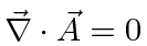 , is often used.
For time dependent conditions, the Lorentz gauge,
, is often used.
For time dependent conditions, the Lorentz gauge,
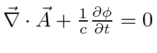 , is often convenient.
These greatly simplify the above wave equations in an obvious way.
, is often convenient.
These greatly simplify the above wave equations in an obvious way.
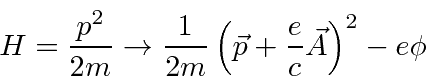
Finally, the classical Hamiltonian for electrons in an electromagnetic field becomes
The magnetic force is not a conservative one so we cannot just add a scalar potential.
We know that there is momentum contained in the field so the additional momentum term, as
well as the usual force due to an electric field, makes sense.
The electron generates an E-field and if there is a B-field present,
 gives rise to momentum density in the field.
The evidence that this is the correct classical Hamiltonian is that we can
derive
the Lorentz Force from it.
gives rise to momentum density in the field.
The evidence that this is the correct classical Hamiltonian is that we can
derive
the Lorentz Force from it.
Jim Branson
2013-04-22